45  Generalized Extreme Value (GEV) Distribution

The Generalized Extreme Value distribution is the universal limiting distribution for block maxima of i.i.d. random variables. By the Fisher-Tippett-Gnedenko theorem, any properly normalized sequence of block maxima that converges in distribution must converge to a GEV — making it the single most important model in extreme-value statistics.

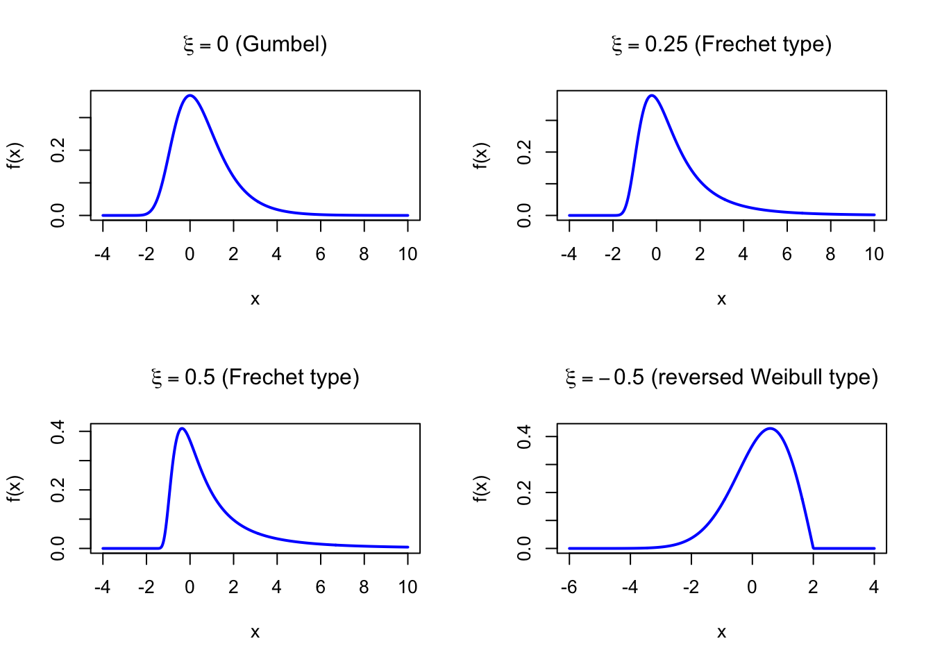
Formally, the random variate \(X\) is said to have a Generalized Extreme Value Distribution (i.e. \(X \sim \text{GEV}(\mu, \sigma, \xi)\)) with location parameter \(\mu \in \mathbb{R}\), scale parameter \(\sigma > 0\), and shape parameter \(\xi \in \mathbb{R}\). The shape parameter \(\xi\) determines the tail behavior and unifies three classical extreme-value types: the Gumbel (\(\xi = 0\)), the Frechet (\(\xi > 0\)), and the reversed Weibull (\(\xi < 0\)). We define \(z = (x - \mu)/\sigma\) throughout this chapter.

45.1 Probability Density Function

\[ f(x) = \frac{1}{\sigma}\bigl(1 + \xi z\bigr)^{-1/\xi - 1}\exp\!\Bigl(-\bigl(1 + \xi z\bigr)^{-1/\xi}\Bigr), \quad 1 + \xi z > 0 \]

For \(\xi = 0\) (Gumbel case), the density reduces by continuity to:

\[ f(x) = \frac{1}{\sigma}\exp\!\bigl(-z - e^{-z}\bigr) \]

The figure below shows examples of the GEV Probability Density Function for different shape parameter values with \(\mu = 0\) and \(\sigma = 1\).

dgev_custom <- function(x, mu, sigma, xi) {
  z <- (x - mu) / sigma
  if (abs(xi) < 1e-8) {
    return(exp(-z - exp(-z)) / sigma)
  }
  t <- 1 + xi * z
  valid <- t > 0
  d <- rep(0, length(x))
  d[valid] <- (1/sigma) * t[valid]^(-1/xi - 1) * exp(-t[valid]^(-1/xi))
  d
}

par(mfrow = c(2, 2))
x <- seq(-4, 10, length = 500)

plot(x, dgev_custom(x, 0, 1, 0), type = "l", lwd = 2, col = "blue",
     xlab = "x", ylab = "f(x)", main = expression(paste(xi == 0, " (Gumbel)")))

plot(x, dgev_custom(x, 0, 1, 0.25), type = "l", lwd = 2, col = "blue",
     xlab = "x", ylab = "f(x)", main = expression(paste(xi == 0.25, " (Frechet type)")))

plot(x, dgev_custom(x, 0, 1, 0.5), type = "l", lwd = 2, col = "blue",
     xlab = "x", ylab = "f(x)", main = expression(paste(xi == 0.5, " (Frechet type)")))

x2 <- seq(-6, 4, length = 500)
plot(x2, dgev_custom(x2, 0, 1, -0.5), type = "l", lwd = 2, col = "blue",
     xlab = "x", ylab = "f(x)", main = expression(paste(xi == -0.5, " (reversed Weibull type)")))

par(mfrow = c(1, 1))

Figure 45.1: GEV Probability Density Function for various shape parameters (location = 0, scale = 1)

45.2 Purpose

The GEV distribution provides a unified framework for extreme-value modeling. Instead of choosing among three separate extreme-value distributions, the analyst fits a single GEV and lets the data determine \(\xi\) — thereby identifying whether the underlying parent has a light tail (\(\xi = 0\), Gumbel), a heavy tail (\(\xi > 0\), Frechet), or a bounded upper tail (\(\xi < 0\), reversed Weibull). Common applications include:

• Flood risk analysis: annual maximum river discharge for dam design
• Extreme temperature modeling: maximum daily temperatures for climate projections
• Financial tail risk: extreme portfolio losses and Value-at-Risk estimation
• Wind speed engineering: maximum wind gusts for structural design codes
• Insurance catastrophe modeling: annual maximum claim sizes

Relation to the discrete setting. The GEV distribution is the continuous limit of the maximum of \(n\) i.i.d. random variables after normalization. There is no single discrete analog, but the Fisher-Tippett-Gnedenko theorem applies to discrete parents as well — the normalized maximum of Geometric, Poisson, or other discrete variates also converges to a GEV after appropriate centering and scaling.

45.3 Distribution Function

\[ F(x) = \exp\!\Bigl(-\bigl(1 + \xi z\bigr)^{-1/\xi}\Bigr), \quad 1 + \xi z > 0 \]

For \(\xi = 0\), this reduces to the Gumbel CDF:

\[ F(x) = \exp\!\bigl(-e^{-z}\bigr) \]

In R (using the evd package): pgev(x, loc = mu, scale = sigma, shape = xi).

The figure below shows the GEV Distribution Function for \(\mu = 0\), \(\sigma = 1\), and \(\xi = 0.25\).

pgev_custom <- function(x, mu, sigma, xi) {
  z <- (x - mu) / sigma
  if (abs(xi) < 1e-8) {
    return(exp(-exp(-z)))
  }
  t <- 1 + xi * z
  valid <- t > 0
  p <- rep(0, length(x))
  p[valid] <- exp(-t[valid]^(-1/xi))
  if (xi < 0) p[!valid & x > mu - sigma/xi] <- 1
  p
}

x <- seq(-4, 12, length = 500)
plot(x, pgev_custom(x, 0, 1, 0.25), type = "l", lwd = 2, col = "blue",
     xlab = "x", ylab = "F(x)", main = "GEV Distribution Function",
     sub = expression(paste(mu == 0, ",  ", sigma == 1, ",  ", xi == 0.25)))

Figure 45.2: GEV Distribution Function (location = 0, scale = 1, shape = 0.25)

45.4 Moment Generating Function

The moment generating function does not exist in closed form for \(\xi > 0\) because the right tail is heavy. For \(\xi = 0\) (Gumbel case):

\[ M_X(t) = \Gamma(1 - \sigma t)\,e^{\mu t}, \quad t < \frac{1}{\sigma} \]

For general \(\xi\), the raw moments are expressed via the gamma function (see below).

45.5 1st Uncentered Moment

\[ \mu_1' = \mu + \frac{\sigma}{\xi}\bigl(\Gamma(1 - \xi) - 1\bigr), \quad \xi < 1, \; \xi \neq 0 \]

For \(\xi = 0\): \(\mu_1' = \mu + \gamma\sigma\), where \(\gamma \approx 0.5772156649\) is the Euler-Mascheroni constant.

45.6 2nd Uncentered Moment

\[ \mu_2' = \mu^2 + \frac{2\mu\sigma}{\xi}\bigl(\Gamma(1-\xi) - 1\bigr) + \frac{\sigma^2}{\xi^2}\bigl(\Gamma(1-2\xi) - 2\Gamma(1-\xi) + 1\bigr), \quad \xi < \tfrac{1}{2} \]

45.7 3rd Uncentered Moment

\[ \mu_3' = \mu^3 + \frac{3\mu^2\sigma}{\xi}\bigl(\Gamma(1-\xi) - 1\bigr) + \frac{3\mu\sigma^2}{\xi^2}\bigl(\Gamma(1-2\xi) - 2\Gamma(1-\xi) + 1\bigr) + \frac{\sigma^3}{\xi^3}\bigl(\Gamma(1-3\xi) - 3\Gamma(1-2\xi) + 3\Gamma(1-\xi) - 1\bigr), \quad \xi < \tfrac{1}{3}, \; \xi \neq 0 \]

45.8 4th Uncentered Moment

Exists only when \(\xi < 1/4\) and involves \(\Gamma(1-k\xi)\) for \(k = 1, 2, 3, 4\).

45.9 2nd Centered Moment

\[ \mu_2 = \frac{\sigma^2}{\xi^2}\bigl(\Gamma(1 - 2\xi) - \Gamma(1-\xi)^2\bigr), \quad \xi < \tfrac{1}{2}, \; \xi \neq 0 \]

For \(\xi = 0\): \(\mu_2 = \dfrac{\pi^2\sigma^2}{6}\).

45.10 3rd Centered Moment

\[ \mu_3 = \frac{\sigma^3}{\xi^3}\bigl(\Gamma(1-3\xi) - 3\,\Gamma(1-2\xi)\,\Gamma(1-\xi) + 2\,\Gamma(1-\xi)^3\bigr), \quad \xi < \tfrac{1}{3} \]

For \(\xi = 0\): \(\mu_3 = 2\zeta(3)\sigma^3\), where \(\zeta(3) \approx 1.20206\).

45.11 4th Centered Moment

\[ \mu_4 = \frac{\sigma^4}{\xi^4}\bigl(\Gamma(1-4\xi) - 4\,\Gamma(1-3\xi)\,\Gamma(1-\xi) + 6\,\Gamma(1-2\xi)\,\Gamma(1-\xi)^2 - 3\,\Gamma(1-\xi)^4\bigr), \quad \xi < \tfrac{1}{4} \]

45.12 Expected Value

\[ \text{E}(X) = \begin{cases} \mu + \dfrac{\sigma}{\xi}\bigl(\Gamma(1-\xi) - 1\bigr) & \xi < 1, \; \xi \neq 0 \\[6pt] \mu + \gamma\sigma & \xi = 0 \end{cases} \]

where \(\gamma \approx 0.5772156649\) is the Euler-Mascheroni constant. For \(\xi \geq 1\), the mean is infinite.

45.13 Variance

\[ \text{V}(X) = \begin{cases} \dfrac{\sigma^2}{\xi^2}\bigl(\Gamma(1-2\xi) - \Gamma(1-\xi)^2\bigr) & \xi < \tfrac{1}{2}, \; \xi \neq 0 \\[6pt] \dfrac{\pi^2\sigma^2}{6} & \xi = 0 \end{cases} \]

For \(\xi \geq 1/2\), the variance is infinite.

45.14 Median

\[ \text{Med}(X) = \begin{cases} \mu + \dfrac{\sigma}{\xi}\bigl((\ln 2)^{-\xi} - 1\bigr) & \xi \neq 0 \\[6pt] \mu - \sigma\ln(\ln 2) & \xi = 0 \end{cases} \]

45.15 Mode

\[ \text{Mo}(X) = \begin{cases} \mu + \dfrac{\sigma}{\xi}\bigl((1 + \xi)^{-\xi} - 1\bigr) & \xi \neq 0 \\[6pt] \mu & \xi = 0 \end{cases} \]

45.16 Coefficient of Skewness

\[ g_1 = \frac{\mu_3}{\mu_2^{3/2}} = \frac{\text{sign}(\xi)\bigl(\Gamma(1-3\xi) - 3\,\Gamma(1-2\xi)\,\Gamma(1-\xi) + 2\,\Gamma(1-\xi)^3\bigr)}{\bigl(\Gamma(1-2\xi) - \Gamma(1-\xi)^2\bigr)^{3/2}}, \quad \xi < \tfrac{1}{3} \]

For \(\xi = 0\) (Gumbel): \(g_1 \approx 1.1395\). For \(\xi > 0\) (Frechet type), the skewness increases as \(\xi\) increases. For \(\xi < 0\) (reversed Weibull type), the skewness decreases.

45.17 Coefficient of Kurtosis

\[ g_2 = \frac{\mu_4}{\mu_2^{2}}, \quad \xi < \tfrac{1}{4} \]

For \(\xi = 0\) (Gumbel): \(g_2 = 5.4\). For \(\xi > 0\), the kurtosis increases rapidly with \(\xi\).

45.18 Parameter Estimation

Maximum likelihood estimation is the standard approach for the GEV. The log-likelihood for a sample \(x_1, \ldots, x_n\) when \(\xi \neq 0\) is:

\[ \ell(\mu, \sigma, \xi) = -n\ln\sigma - \left(1 + \frac{1}{\xi}\right)\sum_{i=1}^n \ln\bigl(1 + \xi z_i\bigr) - \sum_{i=1}^n \bigl(1 + \xi z_i\bigr)^{-1/\xi} \]

subject to \(1 + \xi z_i > 0\) for all \(i\). In R, the evd package provides fgev() for MLE fitting.

library(evd)

set.seed(42)
mu_true <- 10; sigma_true <- 3; xi_true <- 0.2
x_obs <- evd::rgev(200, loc = mu_true, scale = sigma_true, shape = xi_true)

# Maximum likelihood estimation
fit <- evd::fgev(x_obs)
cat("MLE mu:   ", round(fit$estimate["loc"], 4), "\n")
cat("MLE sigma:", round(fit$estimate["scale"], 4), "\n")
cat("MLE xi:   ", round(fit$estimate["shape"], 4), "\n")
cat("True mu:", mu_true, "  True sigma:", sigma_true, "  True xi:", xi_true, "\n")

MLE mu:    9.8084 
MLE sigma: 3.0086 
MLE xi:    0.0455 
True mu: 10   True sigma: 3   True xi: 0.2 

45.19 R Module

45.19.1 RFC

The Generalized Extreme Value Distribution module is available in RFC under the menu “Distributions / Generalized Extreme Value Distribution”.

45.19.2 Direct app link

• https://shiny.wessa.net/gev/

45.19.3 R Code

The following code demonstrates GEV probability calculations using the evd package:

library(evd)

mu <- 10; sigma <- 3; xi <- 0.2

# Probability density function: f(x)
evd::dgev(15, loc = mu, scale = sigma, shape = xi)

# Distribution function: P(X <= x)
evd::pgev(15, loc = mu, scale = sigma, shape = xi)

# Quantile function: 95th percentile (20-year return level)
evd::qgev(0.95, loc = mu, scale = sigma, shape = xi)

# Mean and mode
g1 <- gamma(1 - xi)
cat("Mean:", mu + sigma * (g1 - 1) / xi, "\n")
cat("Mode:", mu + sigma * ((1 + xi)^(-xi) - 1) / xi, "\n")

# Generate random GEV numbers
set.seed(42)
evd::rgev(10, loc = mu, scale = sigma, shape = xi)

[1] 0.04679357
[1] 0.7887509
[1] 22.16934
Mean: 12.46345 
Mode: 9.462888 
 [1] 15.730539 11.295389 14.301159 23.820201 12.421542  8.899692 13.910787
 [8] 12.926976  9.483226 11.041566

45.20 Example

Annual maximum river discharge (m/s) at a gauging station is modeled as \(X \sim \text{GEV}(\mu = 500, \sigma = 100, \xi = 0.2)\). The positive shape parameter indicates heavy-tailed flood behavior (Frechet type). We compute the probability of exceeding a critical discharge threshold and the 100-year return level.

library(evd)

mu <- 500; sigma <- 100; xi <- 0.2

# P(max discharge > 750 m^3/s)
cat("P(discharge > 750):", 1 - evd::pgev(750, loc = mu, scale = sigma, shape = xi), "\n")

# Mean annual maximum discharge
g1 <- gamma(1 - xi)
cat("Mean max discharge:", mu + sigma * (g1 - 1) / xi, "\n")

# 100-year return level (99th percentile)
rl_100 <- evd::qgev(0.99, loc = mu, scale = sigma, shape = xi)
cat("100-year return level:", round(rl_100, 2), "m^3/s\n")

# 50-year return level (98th percentile)
rl_50 <- evd::qgev(0.98, loc = mu, scale = sigma, shape = xi)
cat("50-year return level:", round(rl_50, 2), "m^3/s\n")

P(discharge > 750): 0.1233849 
Mean max discharge: 582.1149 
100-year return level: 1254.68 m^3/s
50-year return level: 1091.16 m^3/s

Interactive Shiny app (click to load).

Open in new tab

45.21 Random Number Generator

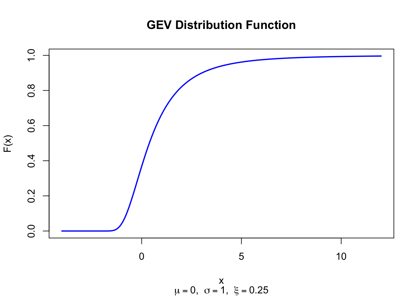
GEV random variates are generated via the inverse-CDF (quantile) method. Since \(F(x) = \exp\!\bigl(-(1 + \xi z)^{-1/\xi}\bigr)\), solving \(U = F(X)\) for \(X\) gives:

\[ X = \begin{cases} \mu + \dfrac{\sigma}{\xi}\bigl((-\ln U)^{-\xi} - 1\bigr) & \xi \neq 0 \\[6pt] \mu - \sigma\ln(-\ln U) & \xi = 0 \end{cases}, \quad U \sim \text{U}(0,1) \]

library(evd)

set.seed(123)
n <- 1000; mu <- 0; sigma <- 1; xi <- 0.25

# Inverse-transform method
u <- runif(n)
x_inv <- mu + (sigma / xi) * ((-log(u))^(-xi) - 1)

cat("Simulated mean:", round(mean(x_inv), 4), "\n")
g1 <- gamma(1 - xi)
cat("Theoretical mean:", round(mu + sigma * (g1 - 1) / xi, 4), "\n")
g2 <- gamma(1 - 2 * xi)
cat("Simulated var:", round(var(x_inv), 4), "\n")
cat("Theoretical var:", round(sigma^2 * (g2 - g1^2) / xi^2, 4), "\n")

Simulated mean: 0.8676 
Theoretical mean: 0.9017 
Simulated var: 3.7123 
Theoretical var: 4.3329 

Interactive Shiny app (click to load).

Open in new tab

45.22 Property 1: Fisher-Tippett-Gnedenko Theorem

The GEV distribution is the only possible non-degenerate limiting distribution for properly normalized block maxima. If \(M_n = \max(X_1, \ldots, X_n)\) for i.i.d. random variables and there exist normalizing sequences \(a_n > 0\) and \(b_n\) such that \((M_n - b_n)/a_n\) converges in distribution to a non-degenerate limit, then that limit must be a GEV distribution for some \(\xi\).

45.23 Property 2: Three Types Unified

The shape parameter \(\xi\) determines the extreme-value type:

• \(\xi = 0\): Gumbel (Type I) — light-tailed parents (Normal, Exponential, Gamma). See Chapter 38.
• \(\xi > 0\): Frechet (Type II) — heavy-tailed parents (Pareto, Student-\(t\), Cauchy). See Chapter 46.
• \(\xi < 0\): Reversed Weibull (Type III) — bounded upper tail (Uniform, Beta). This is the extreme-value family for maxima, not the standard Weibull lifetime distribution.

45.24 Property 3: Max-Stability

The GEV is max-stable: if \(X_1, \ldots, X_n\) are i.i.d. GEV\((\mu, \sigma, \xi)\), then \(\max(X_1, \ldots, X_n)\) is also GEV with the same shape \(\xi\) but updated location and scale:

\[ \max(X_1, \ldots, X_n) \sim \text{GEV}\!\left(\mu + \frac{\sigma}{\xi}(n^\xi - 1),\; \sigma n^\xi,\; \xi\right), \quad \xi \neq 0 \]

45.25 Property 4: Return Levels

The \(T\)-year return level (the value exceeded on average once every \(T\) years) is the \((1 - 1/T)\)-quantile of the GEV:

\[ x_T = \begin{cases} \mu + \dfrac{\sigma}{\xi}\Bigl(\bigl(-\ln(1-1/T)\bigr)^{-\xi} - 1\Bigr) & \xi \neq 0 \\[6pt] \mu - \sigma\ln\bigl(-\ln(1-1/T)\bigr) & \xi = 0 \end{cases} \]

This is the primary quantity of interest in flood frequency analysis, structural wind design, and insurance pricing.

45.26 Related Distributions 1: Gumbel Distribution

The Gumbel distribution is the special case \(\xi = 0\) of the GEV, arising as the limit for light-tailed parent distributions (see Chapter 38).

45.27 Related Distributions 2: Frechet Distribution

The Frechet distribution corresponds to \(\xi > 0\) in the GEV parameterization, arising as the limit for heavy-tailed parent distributions (see Chapter 46).

45.28 Related Distributions 3: Reversed Weibull Family

The reversed Weibull distribution (for maxima) corresponds to \(\xi < 0\) in the GEV, arising from parent distributions with a finite upper endpoint. It is part of extreme-value theory and should not be conflated with the standard Weibull lifetime distribution discussed elsewhere in the handbook.

45.29 Related Distributions 4: Exponential Distribution

The Exponential distribution belongs to the Gumbel (\(\xi = 0\)) domain of attraction: the normalized maximum of \(n\) i.i.d. Exponential variates converges to the Gumbel (and hence GEV with \(\xi = 0\)) as \(n \to \infty\) (see Chapter 27).