156 Transfer Function Noise Models

In Chapter 154, the external input was a binary indicator: an event either happened or it didn’t. But what if the “input” is a continuous, measurable variable — such as the price of raw materials, the interest rate, or the temperature? The transfer function noise model generalises intervention analysis to continuous inputs with dynamic lag structures.

156.1 Motivation

Consider the Coffee dataset: the Colombian import price is a continuous variable that fluctuates over time, and we hypothesise that it influences the US retail price with some delay. A binary intervention variable cannot capture this — we need a model that describes how the entire time path of the input series affects the output series.

The transfer function model answers the question: given a known input series \(X\), how does it dynamically influence the output series \(Y\), after accounting for the ARIMA structure of the noise?
In this chapter we use TF-noise model as the short name for “transfer function noise model.”

156.2 The Transfer Function Model

156.2.1 Model Specification

The general TF-noise model is

\[ Y_t = v(B) X_{t-b} + N_t \]

Its impulse-response expansion is:

\[ v(B)=\sum_{j=0}^{\infty} v_j B^j,\quad v(B)X_{t-b} = \sum_{j=0}^{\infty} v_j X_{t-b-j} \]

In this notation, \(v_j\) are the impulse-response weights; when \(r=0\) (finite impulse response), the sum terminates at \(j=s\).

The model components are:

\(Y_t\) is the output (dependent) series
\(X_t\) is the input (independent) series
\(b\) is the pure delay (dead time) — the number of periods before \(X\) begins to affect \(Y\)
\(v(B)\) is the transfer function that describes the dynamic relationship
\(N_t\) is the noise component, following an ARIMA process

For TF-noise identification, \(X_t\) should be made stationary first (typically by differencing as needed), then used in the prewhitening/CCF workflow.

The transfer function is defined as the ratio of two polynomials in the backshift operator:

\[ v(B) = \frac{\omega(B)}{\delta(B)} = \frac{\omega_0 - \omega_1 B - \omega_2 B^2 - \ldots - \omega_s B^s}{1 - \delta_1 B - \delta_2 B^2 - \ldots - \delta_r B^r} \]

Following Box-Jenkins notation, the numerator is written with negative signs on \(\omega_j\) (\(j\ge 1\)), mirroring the AR-style sign convention in the denominator.

The noise component follows the familiar ARIMA structure:

\[ N_t = \frac{\theta(B)\Theta(B^m)}{\phi(B)\Phi(B^m)(1-B)^d(1-B^m)^D} e_t \]

Combining these, the full model is

\[ Y_t = \frac{\omega_0 - \omega_1 B - \ldots - \omega_s B^s}{1 - \delta_1 B - \ldots - \delta_r B^r} X_{t-b} + \frac{\theta(B)\Theta(B^m)}{\phi(B)\Phi(B^m)(1-B)^d(1-B^m)^D} e_t \]

The parameters \((r, s, b)\) characterise the transfer function: \(b\) is the delay, \(s\) is the order of the numerator (number of input lags), and \(r\) is the order of the denominator (persistence of the effect). Here \(m\) denotes the seasonal period in the ARIMA noise model.
If strong seasonality exists in the transfer channel itself, seasonal factors can also be included in \(v(B)\) (not only in the noise model).

156.2.2 Relationship to Other Models

The TF-noise model is a general framework that includes many familiar models as special cases.

Table 156.1: Special cases of the transfer function model

Special case	Constraint	Reduces to
\(v(B) = \omega_0\), \(N_t\) white noise	No dynamics, no ARIMA noise	OLS regression
\(X_t\) is a binary dummy variable	\(X_t \in \{0,1\}\)	Intervention model (Chapter 154)
\(v(B) = \omega_0\), \(b = 0\)	No lag dynamics	ARIMAX (ARIMA with external regressor)
\(\delta(B) = 1\) (no denominator)	Finite impulse response	Distributed lag model
Full \(v(B)\) with ARIMA noise	General case	TF-Noise (this chapter)

This table shows that the transfer function model provides a unified framework: simple regression, intervention analysis, and ARIMAX are all special cases.

156.3 Impulse-Response Functions

The impulse-response function (IRF) reveals how a transfer function transforms an input signal into an output response. Think of the transfer function as a “black box”: you feed in a known input shape (a pulse, a step, a ramp) and observe what comes out. The shape of the output tells you about the dynamics encoded in \(v(B)\).

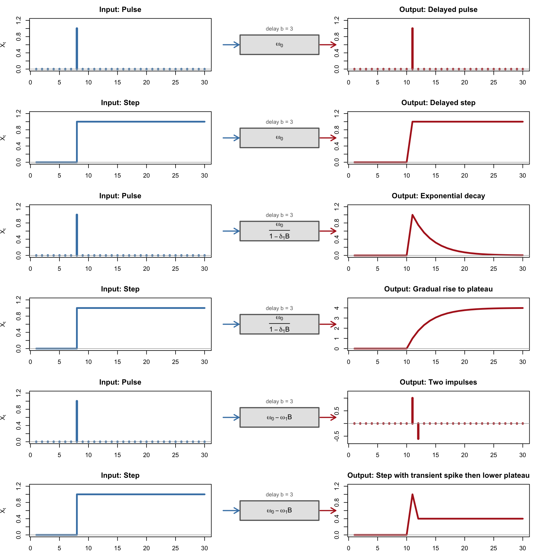
In Section 154.2.2, we saw how binary interventions (pulse or step) produce four response patterns (abrupt/gradual × permanent/temporary). The transfer function generalises this to continuous inputs. The diagrams below show how five common TF orders transform pulse and step inputs — each row places the input on the left, the TF specification in the centre, and the resulting output on the right.

Code

# Layout: 6 rows (2 per case) x 3 columns
layout(matrix(1:18, nrow = 6, ncol = 3, byrow = TRUE),
       widths = c(3, 1.8, 3))

# ============================================================
# Case 1: TF(r=0, s=0, b): v(B) = omega_0  (simple gain)
# ============================================================
w0 <- 1.0

# Pulse -> delayed pulse
y <- rep(0, n)
y[T0 + b] <- w0
draw_irf_row(t, pulse, y, "Pulse", expression(omega[0]),
             "Delayed pulse", "h", "h", b)

# Step -> delayed step
y <- rep(0, n)
y[t >= (T0 + b)] <- w0
draw_irf_row(t, step, y, "Step", expression(omega[0]),
             "Delayed step", "s", "l", b)

# ============================================================
# Case 2: TF(r=1, s=0, b): v(B) = omega_0 / (1 - delta_1 B)
# ============================================================
d1 <- 0.75

# Pulse -> exponential decay
y <- rep(0, n)
start <- T0 + b
for (i in start:n) y[i] <- w0 * d1^(i - start)
draw_irf_row(t, pulse, y, "Pulse",
             expression(frac(omega[0], 1 - delta[1]*B)),
             "Exponential decay", "h", "l", b)

# Step -> gradual rise to plateau
y <- rep(0, n)
for (i in start:n) y[i] <- w0 * (1 - d1^(i - start + 1)) / (1 - d1)
draw_irf_row(t, step, y, "Step",
             expression(frac(omega[0], 1 - delta[1]*B)),
             "Gradual rise to plateau", "s", "l", b)

# ============================================================
# Case 3: TF(r=0, s=1, b): v(B) = omega_0 - omega_1 B
# ============================================================
w1 <- 0.6

# Pulse -> two consecutive impulses
y <- rep(0, n)
y[T0 + b] <- w0
y[T0 + b + 1] <- -w1
draw_irf_row(t, pulse, y, "Pulse",
             expression(omega[0] - omega[1]*B),
             "Two impulses", "h", "h", b)

# Step -> transient spike then lower plateau
y <- rep(0, n)
y[T0 + b] <- w0
for (i in (T0 + b + 1):n) y[i] <- w0 - w1
draw_irf_row(t, step, y, "Step",
             expression(omega[0] - omega[1]*B),
             "Step with transient spike then lower plateau", "s", "l", b)
layout(1)

Figure 156.1: Impulse-response diagrams (Cases 1-3). Each row shows input (left, blue), transfer-function form (centre), and output response (right, red).

Code

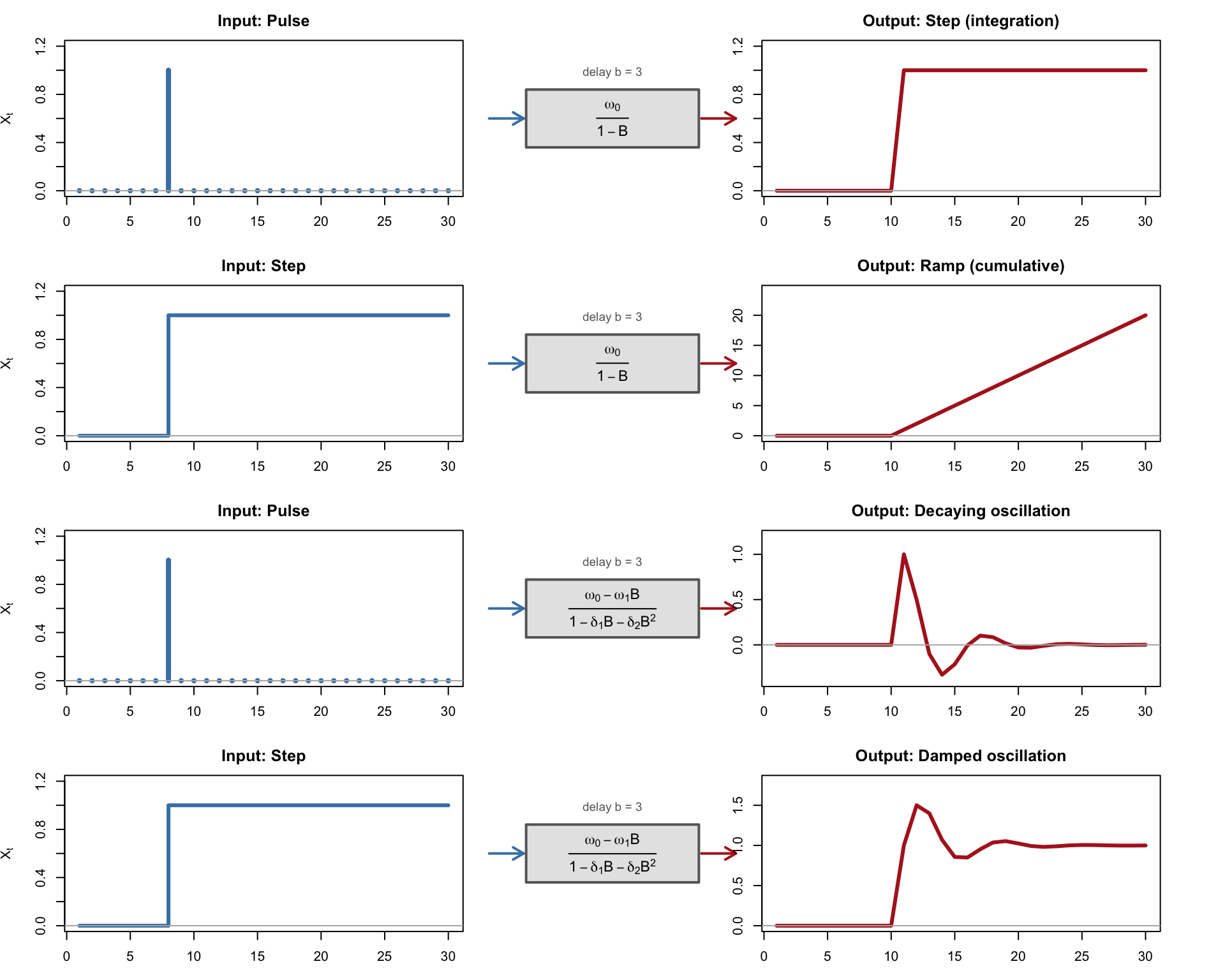
# Layout: 4 rows (2 per case) x 3 columns
layout(matrix(1:12, nrow = 4, ncol = 3, byrow = TRUE),
       widths = c(3, 1.8, 3))

w0 <- 1.0

# ============================================================
# Case 4: Integrating TF: v(B) = omega_0 / (1 - B)
# ============================================================

# Pulse -> step (integration)
y <- rep(0, n)
for (i in (T0 + b):n) y[i] <- w0
draw_irf_row(t, pulse, y, "Pulse",
             expression(frac(omega[0], 1 - B)),
             "Step (integration)", "h", "l", b)

# Step -> ramp (cumulative)
y <- rep(0, n)
for (i in (T0 + b):n) y[i] <- w0 * (i - T0 - b + 1)
draw_irf_row(t, step, y, "Step",
             expression(frac(omega[0], 1 - B)),
             "Ramp (cumulative)", "s", "l", b)

# ============================================================
# Case 5: TF(r=2, s=1, b) with complex roots: oscillatory
# ============================================================
# (w0 - w1 B) / (1 - d1 B - d2 B^2) with complex roots
d1_osc <- 0.8
d2_osc <- -0.5
w1_osc <- 0.3

# Pulse -> damped oscillation
y <- rep(0, n)
# Build impulse response weights first
v <- rep(0, n)
v[1] <- w0
v[2] <- d1_osc * v[1] - w1_osc
for (i in 3:n) v[i] <- d1_osc * v[i-1] + d2_osc * v[i-2]
# Assign impulse-response weights for pulse response
for (i in (T0 + b):n) {
  idx <- i - T0 - b + 1
  y[i] <- v[idx]
}
draw_irf_row(t, pulse, y, "Pulse",
             expression(frac(omega[0] - omega[1]*B,
                             1 - delta[1]*B - delta[2]*B^2)),
             "Decaying oscillation", "h", "l", b)

# Step -> damped oscillation
y <- rep(0, n)
for (i in (T0 + b):n) {
  idx <- i - T0 - b + 1
  y[i] <- sum(v[1:idx])
}
draw_irf_row(t, step, y, "Step",
             expression(frac(omega[0] - omega[1]*B,
                             1 - delta[1]*B - delta[2]*B^2)),
             "Damped oscillation", "s", "l", b)
layout(1)

Figure 156.2: Impulse-response diagrams (Cases 4-5). Each row shows input (left, blue), transfer-function form (centre), and output response (right, red).

These diagrams connect to several earlier concepts:

Cases 1–3 correspond to the CCF patterns in Table 155.1: the prewhitened CCF approximates the impulse response weights \(v_j\).
Case 4 (the integrating system) shows that if the transfer function contains the factor \((1-B)^{-1}\), a stationary input can generate a non-stationary output. The apparent unit-root behavior then comes from the transfer mechanism, not from a unit root in the input itself.
Case 5 shows oscillatory dynamics that arise when the denominator polynomial \(\delta(B)\) has complex roots — the same mechanism that produces pseudo-cyclical behaviour in AR(2) models (Chapter 151).

The intervention response patterns from Section 154.2.2 are the special case where \(X_t\) is a binary pulse or step variable. When \(X_t\) is continuous, the actual output is a convolution of these impulse response weights with the entire input history.

156.4 Model Building Strategy (Box-Jenkins-Tiao)

The Box-Jenkins-Tiao procedure (Box and Jenkins 1970; Tiao and Box 1981) proposes a systematic workflow for building transfer function models. The steps mirror the identification-estimation-diagnostics cycle of the univariate Box-Jenkins methodology.

156.4.1 Step 1: Identify and Estimate ARIMA for X

Fit an ARIMA model to the input series \(X\) using the methods from Chapter 151 and Chapter 152.

156.4.2 Step 2: Prewhiten Both Series

Apply the prewhitening procedure from Section 155.3 to remove autocorrelation and reveal the true cross-correlation structure.

156.4.3 Step 3: Identify Transfer Function via CCF

Examine the prewhitened CCF from Section 155.5 to identify the delay \(b\), numerator order \(s\), and denominator order \(r\). Use the CCF-to-TF mapping in Table 155.1.
Different rational forms can produce very similar CCF signatures (aliasing between numerator and denominator dynamics), so identification is not unique in general.
When several \((r,s,b)\) candidates are plausible, compare them with AIC/BIC and keep the most parsimonious model whose residual diagnostics are indistinguishable from white noise.

156.4.4 Step 4: Estimate Transfer Function

Obtain preliminary estimates of the transfer function parameters. The impulse response weights (the coefficients of \(v(B)\) expanded as a polynomial) can be estimated from the prewhitened CCF.

156.4.5 Step 5: Model the Noise

Compute the residuals from the transfer function:

\[ \hat{N}_t = Y_t - \hat{v}(B) X_{t-b} \]

and identify an ARIMA model for \(\hat{N}_t\) using the standard ACF/PACF analysis.

156.4.6 Step 6: Joint Estimation and Diagnostics

Estimate the transfer function and noise parameters jointly using maximum likelihood. Then perform diagnostic checks:

Residual ACF: Should show no significant autocorrelation (white noise)
CCF of residuals with prewhitened X: Should show no remaining signal
Ljung-Box test (Ljung and Box 1978): Should not reject the null hypothesis of white noise residuals (use fitdf = p + q for ARIMA-noise parameter adjustment)

If diagnostics fail, revise the model (modify \(r\), \(s\), \(b\), or the ARIMA noise order) and re-estimate.

In ARIMAX/TF regressions with many xreg terms, this p+q adjustment is the standard convention, but the test can still be mildly liberal.

156.5 Example: Coffee Prices

We now apply the full transfer function methodology to the Coffee dataset. The input \(X\) is the Colombian import price and the output \(Y\) is the US retail price.

156.5.1 Step 1-3: Identification

Step 1 is shown below. Steps 2 and 3 (prewhitening and CCF analysis) were carried out in Section 155.4; those results motivate the transfer-function specification used here.

# Load the data
coffee <- read.csv("coffee.csv")
colombia <- ts(coffee$Colombia, frequency = 12)
usa <- ts(coffee$USA, frequency = 12)

# Step 1: ARIMA for Colombia
fit_col <- arima(colombia, order = c(1, 1, 1))
cat("ARIMA for Colombia (input):\n")
print(fit_col)

ARIMA for Colombia (input):

Call:
arima(x = colombia, order = c(1, 1, 1))

Coefficients:
          ar1     ma1
      -0.6682  0.7988
s.e.   0.1332  0.1071

sigma^2 estimated as 28.55:  log likelihood = -1111.06,  aic = 2228.12

156.5.2 Step 4-5: Estimation (ARIMAX approach)

While the full TF-noise model requires specialised estimation (e.g. TSA::arimax()), a simpler setup with \(v(B)=\omega_0\) (no dynamic lag polynomial, contemporaneous effect only) can be estimated directly with R’s arima() function using xreg.

Important terminology note: in strict time-series notation, stats::arima(..., xreg=...) is regression with ARIMA errors. In applied workflows this is often called ARIMAX. In this chapter we use the shorthand “ARIMAX” for that implementation, while the full model with transfer polynomials is referred to as the TF-noise model.

# ARIMAX (in the applied shorthand): regression with ARIMA errors
# for USA using Colombia as external regressor.
# Here xreg is the contemporaneous level of Colombia.
# In this implementation, ARIMA operators are estimated jointly with the regression.
fit_arimax <- arima(usa, order = c(1, 1, 1),
                    xreg = as.numeric(colombia))
cat("ARIMAX: USA = f(Colombia) + ARIMA noise:\n")
print(fit_arimax)

ARIMAX: USA = f(Colombia) + ARIMA noise:

Call:
arima(x = usa, order = c(1, 1, 1), xreg = as.numeric(colombia))

Coefficients:
         ar1     ma1  as.numeric(colombia)
      0.2463  0.2241                0.0931
s.e.  0.1488  0.1542                0.1021

sigma^2 estimated as 111.8:  log likelihood = -1356.2,  aic = 2720.4

# Match the embedded app setup:
# ARIMA(3,1,0) noise with a finite transfer function TF(r=0,s=4,b=0),
# where s=4 means coefficients on lags 0..4 (five terms total).
n <- length(colombia)
xreg_lagged <- cbind(
  col_lag0 = as.numeric(colombia),
  col_lag1 = c(NA, as.numeric(colombia[-n])),
  col_lag2 = c(NA, NA, as.numeric(colombia[-c(n-1, n)])),
  col_lag3 = c(NA, NA, NA, as.numeric(colombia[-c(n-2, n-1, n)])),
  col_lag4 = c(NA, NA, NA, NA, as.numeric(colombia[-c(n-3, n-2, n-1, n)]))
)

# Trim the NAs induced by lagging
start_idx <- 5
fit_tf <- arima(usa[start_idx:n],
                order = c(3, 1, 0),
                xreg = xreg_lagged[start_idx:n, ])
cat("ARIMA(3,1,0) with lagged Colombia inputs (lags 0..4):\n")
print(fit_tf)

ARIMA(3,1,0) with lagged Colombia inputs (lags 0..4):

Call:
arima(x = usa[start_idx:n], order = c(3, 1, 0), xreg = xreg_lagged[start_idx:n, 
    ])

Coefficients:
         ar1      ar2     ar3  col_lag0  col_lag1  col_lag2  col_lag3  col_lag4
      0.3404  -0.1612  0.0147    0.2498    0.3497    0.3866    0.3025    0.2088
s.e.  0.0555   0.0572  0.0580    0.1034    0.1062    0.1123    0.1042    0.1041

sigma^2 estimated as 101.1:  log likelihood = -1323.18,  aic = 2664.37

156.5.3 Step 6: Diagnostics

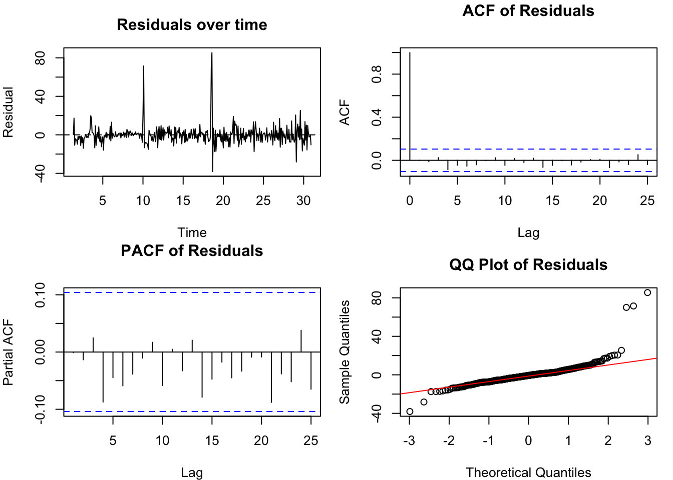
resid_tf <- residuals(fit_tf)
resid_tf_ts <- ts(resid_tf, start = time(usa)[start_idx], frequency = frequency(usa))

par(mfrow = c(2, 2), mar = c(4, 4, 3, 1))
plot(resid_tf_ts, main = "Residuals over time", ylab = "Residual", xlab = "Time")
abline(h = 0, lty = 2)
acf(resid_tf, main = "ACF of Residuals", na.action = na.pass)
pacf(resid_tf, main = "PACF of Residuals", na.action = na.pass)
qqnorm(resid_tf, main = "QQ Plot of Residuals")
qqline(resid_tf, col = "red")
par(mfrow = c(1, 1))

cat("\nLjung-Box test:\n")
print(Box.test(resid_tf, lag = 24, type = "Ljung-Box", fitdf = 3))


Ljung-Box test:

    Box-Ljung test

data:  resid_tf
X-squared = 13.737, df = 21, p-value = 0.8806

Figure 156.3: Diagnostics for the Coffee transfer function model

156.5.4 Comparison: Pure ARIMA vs ARIMAX

# Pure ARIMA for USA
fit_pure <- arima(usa, order = c(1, 1, 1))

cat("AIC comparison:\n")
cat("  Pure ARIMA:  ", AIC(fit_pure), "\n")
cat("  ARIMAX:      ", AIC(fit_arimax), "\n")
cat("  TF-lag model:", AIC(fit_tf), " (estimated on trimmed sample usa[5:n])\n")
cat("\nThe ARIMAX model has a",
    ifelse(AIC(fit_arimax) < AIC(fit_pure), "lower", "higher"),
    "AIC, indicating a",
    ifelse(AIC(fit_arimax) < AIC(fit_pure), "better", "worse"),
    "fit.\n")
cat("Note: the TF-lag model AIC is not directly comparable to the two values above because lagged regressors require trimming the first four observations.\n")

AIC comparison:
  Pure ARIMA:   2719.242 
  ARIMAX:       2720.401 
  TF-lag model: 2664.37  (estimated on trimmed sample usa[5:n])

The ARIMAX model has a higher AIC, indicating a worse fit.
Note: the TF-lag model AIC is not directly comparable to the two values above because lagged regressors require trimming the first four observations.

Note

The embedded app below is preconfigured to reproduce the chapter setup: target = USA, input = Colombia, ARIMA noise = (3,1,0), and transfer-function orders (r,s,b) = (0,4,0). This implies an immediate effect plus four additional lag terms (lags 0 through 4). If the app opens on a different model tab, switch to the TF tab first.

Interactive Shiny app (click to load).

Open in new tab

156.6 Forecasting with Transfer Functions

To forecast \(Y\) using a transfer function model, you need future values of \(X\) (or forecasts of \(X\)). This is a fundamental difference from pure ARIMA forecasting, which only requires the past of \(Y\).

\[ \hat{Y}_{T+h} = \sum_{j=0}^{\infty} \hat{v}_j X_{T+h-b-j} + \hat{N}_{T+h} \]

For small horizons some required \(X_{T+h-b-j}\) values may already be observed; for larger horizons they are future values and must be forecasted unless known by design (contracts, policy paths), which adds uncertainty.

To make this distinction explicit, we run two forecast experiments with the same model structure and only change the cutoff date.
For these forecasting demonstrations we intentionally use a parsimonious ARIMA(1,1,1) noise setup for all compared models to keep the three forecast curves directly comparable in short holdout windows; this differs from the richer estimation example above (ARIMA(3,1,0) with lagged inputs), which is optimized for in-sample explanatory fit.

Stress-test cutoff near the major jump (time 18.0): this isolates how much forecast quality depends on knowing future input values.
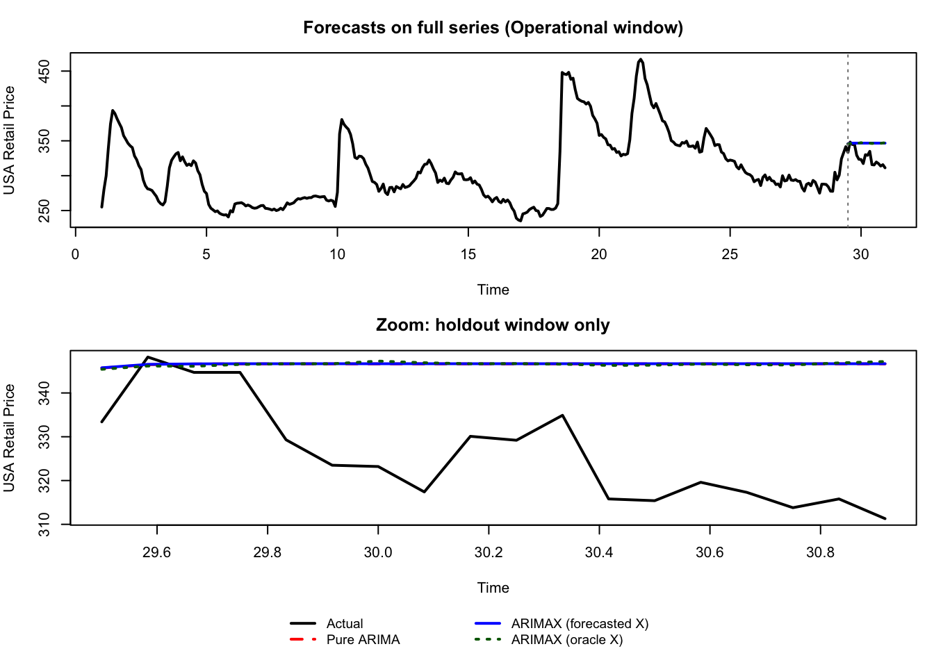
Operational cutoff in a calmer segment (time 29.5): this shows what the same models look like in routine forecasting conditions.

In each experiment we compare:

Pure ARIMA on USA only,
ARIMAX (forecasted X) using forecasts of Colombia (realistic deployment),
ARIMAX (oracle X) using actual future Colombia: an unachievable benchmark that isolates the information value of perfect foresight for the exogenous series.

156.6.1 Experiment A: Stress-Test Cutoff at the Major Jump

This split is intentionally severe. It answers: if the exogenous series moves abruptly right after the cutoff, how much can we gain from knowing future input values?

run_tf_experiment(cutoff_time = 18.0, scenario_label = "Stress test")


Stress test (cutoff = 18)
Mean Absolute Error:
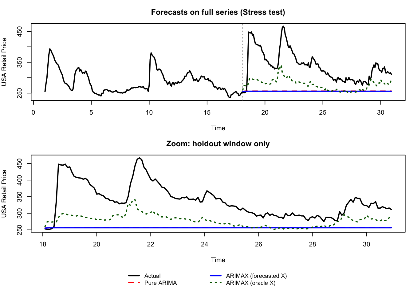
  Pure ARIMA: 81.75 
  ARIMAX (forecasted X): 82.05 
  ARIMAX (oracle X):     61.14 
Input-information gap |oracle - forecasted X|:
  Mean absolute gap: 22.38 
  Maximum gap:       84.47

Figure 156.4: Stress-test forecasting experiment (cutoff = 18.0): pure ARIMA, ARIMAX with forecasted input, and ARIMAX with oracle input.

In this stress-test, the gap between ARIMAX (oracle X) and ARIMAX (forecasted X) mainly measures information loss from not observing future Colombia. This is a pedagogical upper-bound check, not the default production setting.

156.6.2 Experiment B: Operational Cutoff in a Calmer Segment

This split uses a later cutoff where the immediate post-cutoff segment is less dominated by a structural jump. It answers: under routine conditions, how visible is the exogenous effect in actual forecast curves?

run_tf_experiment(cutoff_time = 29.5, scenario_label = "Operational window")


Operational window (cutoff = 29.5)
Mean Absolute Error:
  Pure ARIMA: 20.8 
  ARIMAX (forecasted X): 20.82 
  ARIMAX (oracle X):     20.79 
Input-information gap |oracle - forecasted X|:
  Mean absolute gap: 0.25 
  Maximum gap:       0.6

Figure 156.5: Operational forecasting experiment (cutoff = 29.5): same model class under a calmer holdout window.

Why A Small Curve Gap Can Still Matter

In Experiment B, the forecast curves can look almost identical. That does not imply zero business value.

Statistical differences in levels may be small, but operational decisions are taken at scale (volumes, contracts, inventory positions).
Forecast value should be judged through a business loss function, not by visual distance alone.
This is the same decision logic used in ROC analysis: optimize expected payoff, not only statistical significance (Section 60.5, Section 60.8).

If \(e_t^{(0)}\) and \(e_t^{(1)}\) are forecast errors from two models and \(L(\cdot)\) is the monetary loss per period, the relevant quantity is:

\[ \Delta \text{Value} = \sum_{t=1}^{H} \left[L\!\left(e_t^{(0)}\right) - L\!\left(e_t^{(1)}\right)\right]. \]

When under-forecasting and over-forecasting have asymmetric costs (stockouts, emergency procurement, spoilage), even a small MAE improvement can generate a large positive \(\Delta \text{Value}\).

156.6.3 Experiment C: Hands-On Window with Strong Lead Signal

The previous two experiments (A and B) were fixed forecasting comparisons.
Experiment C now switches to a guided lab exercise: use a local prewhitened CCF signal to choose a lead and test whether that lead materially improves extrapolation in that specific window.

Because this workflow is interactive and currently not fully bookmark-reproducible, treat it as a guided laboratory exercise with expected approximate outputs.

The built-in Coffee data has no calendar column; the selected local window (rows 113--233) is therefore referenced by row index and corresponds to a contiguous subperiod of the 360 monthly observations (roughly time index 10.33 to 20.33 in the chapter’s ts(..., frequency = 12) scale).

156.6.3.1 Step-by-Step Procedure

In the CCF/prewhitening app, set X = Colombia, Y = USA, and use the local sample window rows 113--233 (monthly frequency 12).
Configure prewhitening as in your setup (ARMA(3,3) on transformed X, effective ARIMA(3,1,3), D=0); this order is used here because it yields an acceptably whitened local X residual series in this window.
Inspect the prewhitened CCF: identify a meaningful lead at approximately k = -5 (R convention: negative lag means X leads Y).
Open the Manual Model Building app from the menu Models / Manual Model Building and go to the TF tab.
Keep the same sample range (rows 113--233) and split (Training set % = 0.9).

In this section, extrapolation \(R^2\) means holdout-period \(R^2 = 1 - SS_{\text{res}}/SS_{\text{tot}}\), computed on the out-of-sample window.

Once in the app, complete this model comparison:

Fit the baseline ARIMA on USA only (no exogenous variable selected) and record extrapolation \(R^2\).
Go to the Input tab and create lagged regressors explicitly: set Numeric Column = Colombia, set Create Variable = first 12 lags; this creates Colombia_1, ..., Colombia_12 including Colombia_5.
Return to the TF tab, select variables USA and Colombia_5, keep transfer settings (r,s,b) = (0,0,0) for this lagged regressor, and re-estimate.
Record the new extrapolation \(R^2\) and compare with baseline.

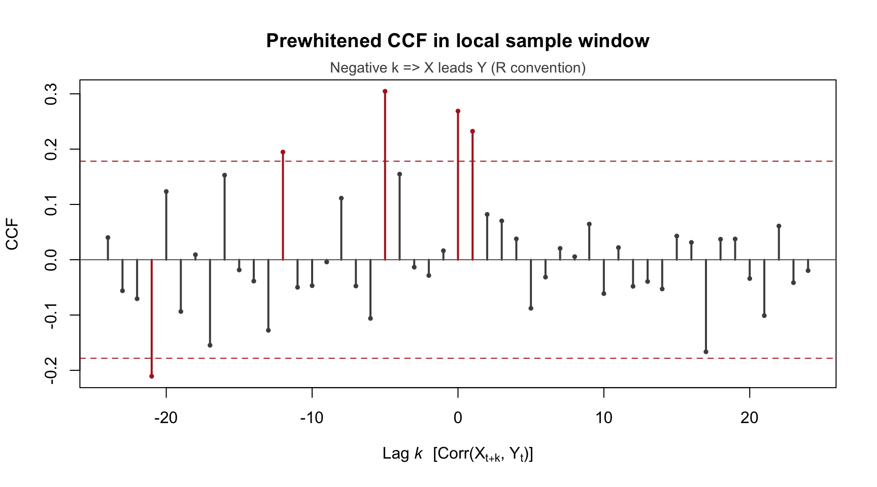
A representative prewhitened CCF for this local window is shown below (same sample range and model order used in this hands-on workflow):

idx <- 113:233
x_win <- as.numeric(coffee$Colombia[idx])
y_win <- as.numeric(coffee$USA[idx])

# Local prewhitening setup used for the hands-on experiment
# 1) Fit filter on X
fit_x_pw <- arima(x_win, order = c(3, 1, 3), include.mean = FALSE, method = "ML")

# 2) Apply the same estimated filter to Y (canonical Box-Jenkins prewhitening)
coef_x <- coef(fit_x_pw)[grepl("^(ar|ma)[0-9]+$", names(coef(fit_x_pw)))]
fit_y_pw_same_filter <- arima(
  y_win,
  order = c(3, 1, 3),
  include.mean = FALSE,
  fixed = as.numeric(coef_x),
  transform.pars = FALSE,
  method = "ML"
)

rx <- residuals(fit_x_pw)
ry <- residuals(fit_y_pw_same_filter)
ok <- is.finite(rx) & is.finite(ry)
rx <- rx[ok]
ry <- ry[ok]

cc <- ccf(rx, ry, lag.max = 24, plot = FALSE, na.action = na.omit)
lags <- as.numeric(cc$lag)
vals <- as.numeric(cc$acf)
n_eff <- length(rx)
bound <- 1.96 / sqrt(n_eff)
sig <- abs(vals) > bound

plot(lags, vals, type = "h", lwd = 2,
     col = ifelse(sig, "firebrick", "grey30"),
     xlab = expression(paste("Lag ", italic(k), "  [Corr(", X[t+k], ", ", Y[t], ")]")),
     ylab = "CCF",
     main = "Prewhitened CCF in local sample window")
points(lags, vals, pch = 16, cex = 0.65,
       col = ifelse(sig, "firebrick", "grey30"))
abline(h = 0, col = "grey40")
abline(h = c(-bound, bound), col = "firebrick", lty = 2)
mtext("Negative k => X leads Y (R convention)", side = 3, line = 0.2, cex = 0.9, col = "grey30")

Figure 156.6: Experiment C local-window prewhitened CCF (rows 113–233). Spikes beyond the approximate ±1.96/sqrt(n_eff) bounds are highlighted.

Why this construction instead of entering lag via (r,s,b) directly?

For this hands-on extrapolation exercise, the current interface behaves more reliably when the lead is encoded as an explicit lagged input variable.
Using Colombia_5 with r=s=b=0 is equivalent to a single-delay transfer term (a pure lag-5 effect with no distributed lag polynomial), but it keeps train/test extrapolation fully transparent in the app workflow.
At forecast origin \(t\), Colombia_5(t) = Colombia(t-5) is already observed; this is exactly why a 5-month lead can be operationally exploitable.
This is a practical implementation choice for reproducible classroom experiments, not a theoretical restriction of transfer-function models.

So Experiment C is a lagged-ARIMAX/single-delay transfer exercise, not a full TF-noise polynomial fit with jointly estimated \((r,s,b)\).

156.6.3.2 Expected Checkpoint Table (Approximate)

Checkpoint	What you should observe (approx.)	Interpretation
Prewhitened CCF local lead	significant spike around `k = -5`	Local evidence that `Colombia` leads `USA` by about 5 months
Baseline ARIMA extrapolation \(R^2\)	\(\approx 0.49\)	Moderate out-of-sample fit in this window
Lagged-ARIMAX (single-delay `Colombia_5`) extrapolation \(R^2\)	\(\approx 0.87\)	Large gain when lead information is explicitly modeled
Incremental gain \(\Delta R^2\)	\(\approx +0.38\)	Exogenous effect is operationally relevant in this regime

Small numerical differences are expected across software/runtime environments; use the table as a calibration band, not a strict equality check.
Also note the window was selected for pedagogical illustration of a visible local lead signal; validate on additional windows to avoid selection bias.

This is intentionally a window-specific result: it reinforces that transfer effects and their practical value are not constant over time. It therefore complements Experiment A (high-shock stress test) and Experiment B (calmer operational segment).

Taken together, the three experiments separate three complementary concepts:

Model mechanism (stress-test): the transfer-function channel can matter materially when future input information is available.
Operational visibility (calmer cutoff): with realistic input forecasts and moderate pass-through, curve differences can be small and must be assessed quantitatively (MAE and gap statistics), not only visually.
Regime dependence (hands-on local window): the relevance of exogenous transfer effects can vary strongly over time.

156.7 Purpose, Pros & Cons

Purpose: Transfer function noise models allow the analyst to model the dynamic influence of a continuous input series on an output series, while accounting for the ARIMA structure of the remaining noise.

Advantages:

Provides a principled framework for incorporating external information
Captures lead/lag dynamics that simple regression cannot
Unifies regression, intervention analysis, and ARIMA in a single model
Can improve forecasting accuracy when the input series is known or predictable

Limitations:

Requires that future values of \(X\) are known or can be forecasted
Assumes a linear, time-invariant relationship between \(X\) and \(Y\)
The identification of \((r,s,b)\) from the CCF can be ambiguous in practice because different transfer structures can imply near-equivalent impulse responses (identifiability/aliasing), so model discrimination must rely on parsimony plus residual diagnostics
Full TF-noise estimation requires specialised software (e.g. TSA::arimax())
Limited to a single input series (extensions to multiple inputs are possible but more complex)
Assumes a unidirectional causal flow from \(X\) to \(Y\) in the standard forecasting setup (no lead terms, \(b \ge 0\)). If the prewhitened CCF shows significant spikes on both sides of lag zero (as in the Coffee example, Section 155.4), this may indicate feedback or anticipation effects that are better handled by a VAR or error-correction model (Section 157.3) with bidirectional dynamics.

156.8 Tasks

Simplify the transfer function model by setting \(r = 0\) (no denominator — a finite impulse response model). Fit the model using arima() with several lagged values of Colombia as xreg. How does the fit compare to the model with a denominator?
Reverse the roles: model Colombia as a function of USA retail prices. Does the model work? How does its fit compare to the original direction? Is this consistent with the Granger causality results from Section 155.6?
Compare the forecasting accuracy of the following models for the last 24 months of USA retail prices: (a) pure ARIMA, (b) ARIMAX with contemporaneous Colombia only, (c) ARIMAX with lagged Colombia. Which is most accurate and why?
Interactive: Open the Manual Model Building app from the menu Models / Manual Model Building, go to the TF tab, and check the settings: target USA, input Colombia, ARIMA noise (3,1,0), and TF orders (r,s,b)=(0,4,0). Compare the coefficient estimates with the R output from Step 4–5 above. Do they match?