Many model settings are not estimated automatically from the data. They must be fixed before fitting begins. Those settings are hyperparameters.
Examples from this handbook include:
Method
Hyperparameter examples
Ridge / lasso / elastic net
lambda, alpha
Conditional random forest
ntree, mtry, mincriterion
Naive Bayes
Laplace correction, kernel choice
k-nearest neighbors
k
Smoothing methods
bandwidth or window width
The central rule is simple: hyperparameters should be chosen by validation, not by convenience.
162.1 Why Hyperparameter Tuning Is a Modeling Stage
Hyperparameter optimization is not an optional technical afterthought. It is one of the main modeling decisions.
If you make the model too flexible, it overfits. If you make it too rigid, it underfits. Tuning is the search for a defensible middle ground.
That is why the tuning stage belongs inside the larger workflow described in Section 158.1:
define the goal,
split the data honestly,
search over candidate settings,
compare held-out performance,
choose a setting,
only then report final performance on untouched data if such a split has been reserved.
162.2 Common Search Strategies
Strategy
Idea
Strength
Weakness
Manual tuning
try a few values by judgment
fast for teaching and small problems
can miss good regions entirely
Grid search
define a small grid and evaluate every combination
transparent and reproducible
becomes expensive as dimensions grow
Random search
sample settings at random from a sensible range
more efficient when many hyperparameters exist
less exhaustive, can feel less intuitive
Adaptive search
use previous results to guide the next trial
efficient for expensive models
harder to explain and audit
For this handbook, grid search is the best teaching device because students can see every candidate value and every comparison. In larger real-world problems, random or adaptive search often becomes more practical.
162.3 A Tuning Workflow That Stays Honest
The search itself can cause optimism if the same data are reused carelessly. The safe pattern is:
use the training data to fit the candidate settings,
use validation or repeated holdout to compare those settings,
keep a separate outer test or locked final test for one last report if the workflow is confirmatory.
This is the same discipline used in Chapter 161. The object being tuned changes; the logic does not.
162.4 Worked Example: Tuning cforest on Pima.tr
The current manual app now lets you fit cforest directly, but it does not expose a full search grid. The point of this chapter is therefore to show the search explicitly in R.
We tune two forest hyperparameters:
ntree: how many trees are averaged,
mtry: how many predictors are considered at each split.
To keep the example readable, the grid is deliberately small and each setting is evaluated across five repeated holdout splits.
Repeated-holdout AUC for a small cforest hyperparameter grid
ntree
mtry
mean_auc
sd_auc
6
200
3
0.881
0.048
8
100
4
0.855
0.041
1
50
2
0.822
0.061
2
100
2
0.820
0.051
3
200
2
0.819
0.025
5
100
3
0.817
0.057
4
50
3
0.805
0.063
7
50
4
0.792
0.034
9
200
4
0.792
0.047
162.4.1 Visualizing Accuracy and Reliability Together
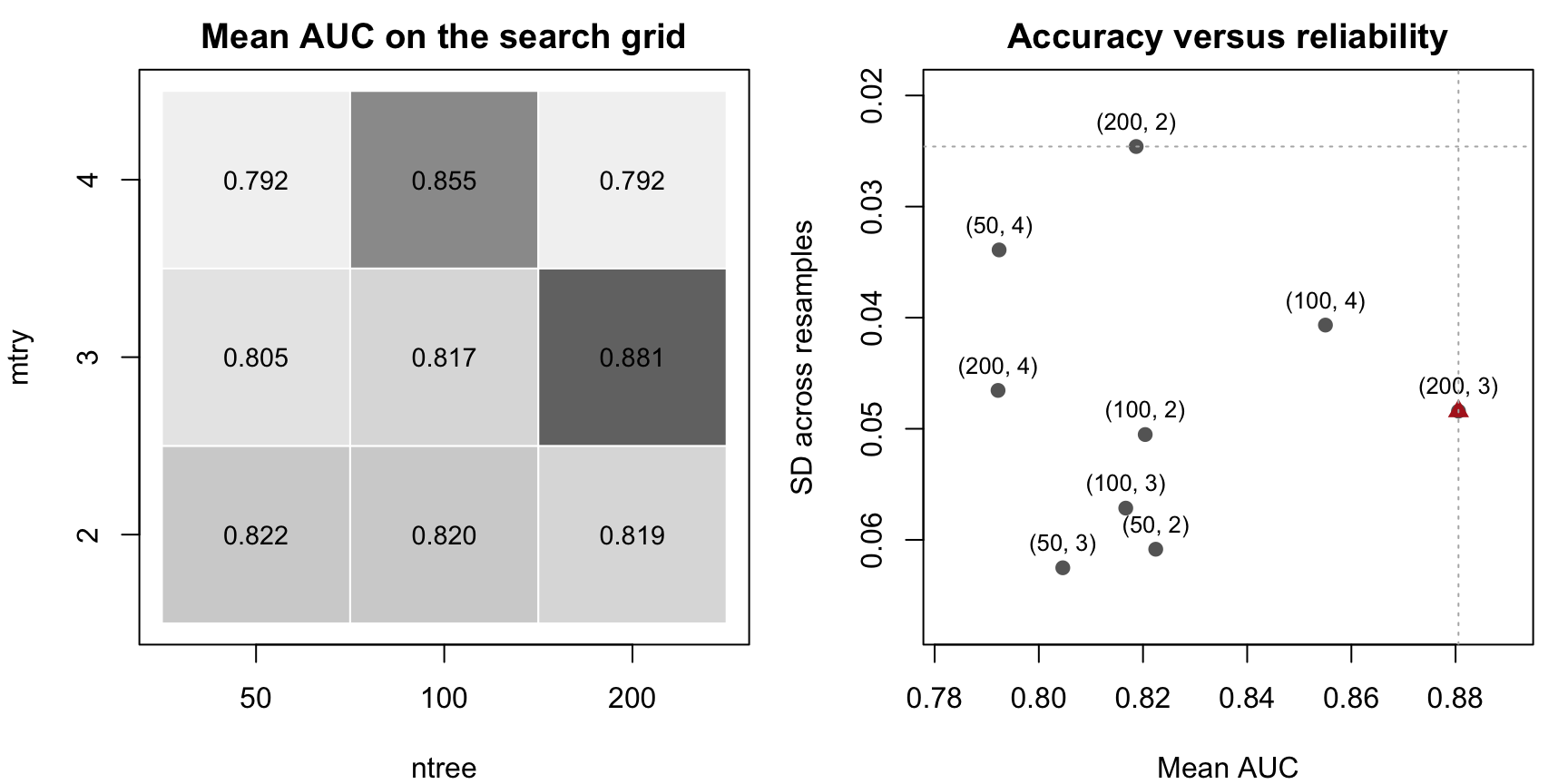
The next figure uses the same tuning results in two ways:
the left panel shows mean AUC on the grid,
the right panel shows the tradeoff between average AUC and variability across resamples.
ntree_vals <-sort(unique(forest_grid$ntree))mtry_vals <-sort(unique(forest_grid$mtry))mean_mat <-matrix(NA_real_,nrow =length(mtry_vals),ncol =length(ntree_vals),dimnames =list(mtry_vals, ntree_vals))for (i inseq_len(nrow(forest_grid))) { row_idx <-match(forest_grid$mtry[i], mtry_vals) col_idx <-match(forest_grid$ntree[i], ntree_vals) mean_mat[row_idx, col_idx] <- forest_grid$mean_auc[i]}zvals <-as.vector(mean_mat)zbreaks <-seq(min(zvals) -1e-6, max(zvals) +1e-6, length.out =11)zcols <-gray.colors(length(zbreaks) -1, start =0.95, end =0.45)par(mfrow =c(1, 2), mar =c(4, 4, 2, 1))plot.new()plot.window(xlim =c(0.5, length(ntree_vals) +0.5),ylim =c(0.5, length(mtry_vals) +0.5))for (i inseq_along(ntree_vals)) {for (j inseq_along(mtry_vals)) { val <- mean_mat[j, i] col_idx <-findInterval(val, zbreaks, all.inside =TRUE)rect(i -0.5, j -0.5, i +0.5, j +0.5,col = zcols[col_idx], border ="white")text(i, j, labels =sprintf("%.3f", val), cex =0.9) }}axis(1, at =seq_along(ntree_vals), labels = ntree_vals)axis(2, at =seq_along(mtry_vals), labels = mtry_vals)box()title(main ="Mean AUC on the search grid",xlab ="ntree",ylab ="mtry")best_idx <-which.max(forest_grid$mean_auc)plot(forest_grid$mean_auc, forest_grid$sd_auc,xlab ="Mean AUC",ylab ="SD across resamples",main ="Accuracy versus reliability",pch =19, col ="grey40",xlim =c(min(forest_grid$mean_auc) -0.01, max(forest_grid$mean_auc) +0.01),ylim =c(max(forest_grid$sd_auc) +0.005, min(forest_grid$sd_auc) -0.005))text(forest_grid$mean_auc, forest_grid$sd_auc,labels =paste0("(", forest_grid$ntree, ", ", forest_grid$mtry, ")"),pos =3, cex =0.8)points(forest_grid$mean_auc[best_idx], forest_grid$sd_auc[best_idx],pch =17, col ="firebrick", cex =1.2)abline(v =max(forest_grid$mean_auc), lty =3, col ="grey70")abline(h =min(forest_grid$sd_auc), lty =3, col ="grey70")
Hyperparameter tuning for cforest on Pima.tr. Left: mean AUC on a small ntree × mtry grid. Right: average AUC versus variability across resamples.
The right-hand panel is especially important. The point with the highest mean AUC is not always the point with the lowest variability.
That gives two different questions:
Which setting is best on average?
Which setting is most reliable across resamples?
If one setting is clearly better on both, the decision is easy. If one setting is slightly better on average but much more variable, the decision becomes a judgment call rather than a mechanical rule.
162.5 How to Read Near Ties
Hyperparameter search almost never ends with one magical number. More often, several settings are practically close.
When settings are close, use a rule like this:
prefer the higher average performance,
but do not ignore variability,
and if the gap in mean performance is tiny, prefer the simpler or cheaper setting.
For a forest, “simpler or cheaper” can mean:
fewer trees,
smaller mtry,
or a setting whose performance is almost as good but clearly more stable.
This is the same reasoning used in the predictive-stability plots of the Guided Model Building app. The vocabulary changes from chapter to chapter, but the workflow principle stays the same: average accuracy and reliability are both part of model quality.
162.6 Beyond Grid Search
The toy grid above is useful because it is small enough to inspect completely. In larger problems, full grids become inefficient.
That is where random search becomes attractive. If a model has several hyperparameters, a coarse grid can waste many fits on unimportant directions, while random search can explore more of the space with the same computational budget.
So the practical progression is:
use grid search when the teaching goal is transparency,
use random or adaptive search when the real-world problem becomes too large for exhaustive grids.
162.7 Try Hyperparameter Tuning in the Apps
The apps now expose two different tuning styles:
the app in the menu Models / Manual Model Building gives you direct control over specific hyperparameters such as ntree, mtry, and the regularization mode,
the Guided Model Building app automates compact training-only searches for regularized coefficient models and then reports the selected tuning summary inside the workflow.
162.7.1 Manual Model Building: Explicit cforest Controls
In the manual app, the Tree tab now lets you switch between ctree and cforest, choose a capped number of trees, set mtry, and fit the forest asynchronously. If another heavy forest fit is already running, the app places the request in a simple queue and tells the learner to wait instead of hammering the fit button repeatedly.
That is not a full grid search, but it is a genuine hyperparameter exercise: you can change the forest size, change mtry, refit, and compare how the confusion matrix, threshold-sensitive metrics, ROC behavior, and forest importance output respond.
162.7.2 Guided Model Building: Automated Shrinkage Tuning
The guided app does not expose a large open search grid. Instead, it automates a compact search over ridge, elastic-net, and lasso style penalties for its regularized coefficient candidates and reports the resulting summary in the fitted model details.
WarningFull-screen use
The Guided Model Building app still works best in a new tab, but the embedded session below opens directly on a regularized Cars93 workflow so you can inspect the tuned search table and the predictive-stability plots.
Interactive Guided Model Building session (click to load).
the guided app keeps the search smaller and more structured, but still shows which hyperparameter choice won and how stable that choice looks across validation splits.
What the apps still do not do is let the learner launch a very large free-form search across many model families at once. This chapter therefore remains useful because it shows the larger logic of search grids, repeated evaluation, and the tradeoff between average performance and reliability.
162.8 Practical Reading Rule
Treat hyperparameter optimization as part of the model, not as a cosmetic setting panel.
Never tune on the final test data.
Prefer validation summaries over training scores.
Read both average performance and variability.
When two settings are practically tied, prefer the simpler or cheaper one.
162.9 Practical Exercises
Extend the cforest grid by adding ntree = 300. Does the best mean AUC improve enough to justify the extra computation?
Change the evaluation metric from AUC to accuracy at threshold 0.50. Does the ranking of the grid change?
Repeat the same tuning exercise with only mtry = 2 and many different ntree values. At what point does adding more trees stop helping much?
Write one paragraph explaining why a final untouched test set is still useful even after a large validation-based search.