135  Multiple Linear Regression Model (MLRM)

The Multiple Linear Regression Model is a generalization of the Simple Linear Regression Model that was described in the previous sections.

The mathematical treatment of the Simple Linear Regression Model was based upon “standard” algebra. Due to the complexity of the Multiple Regression Model, it is necessary to make use of Elementary Matrix Algebra (cfr. Appendix D) such that the formal derivations remain compact - hence more “readable”.

The multiple regression model is explained in the context of two statistical approaches:

• the Ordinary Least Squares approach to multiple regression
• the Maximum Likelihood Estimation approach to multiple regression

Terminology note: “exogenous/endogenous” in this chapter is equivalent to “predictor/response” used in the later applied chapters.

135.1 Ordinary Least Squares for Multiple Linear Regression

135.1.1 Model

The MLRM can be described in matrix notation as

\[ y = X \beta + e \]

where \(y\) is a stochastic \(n \times 1\) vector, \(X\) is a deterministic (exogenous) \(n \times k\) matrix, \(\beta\) is a \(k \times 1\) vector of invariant parameters to be estimated by OLS, \(e\) is a \(n \times 1\) disturbance vector, \(n\) is the number of observations in the sample, and \(k\) is the number of exogenous variables used in the right hand side of the equation. Note: the constant term is coded by a column in matrix \(X\) which only contains the value 1.

It is furthermore assumed that

\[ \begin{cases}\text{E}(y) = \text{E}(X \beta) + \text{E}(e) = X \beta \\\text{E}[(y-\text{E}(y))(y-\text{E}(y))'] = \text{E}(e e') = \sigma^2 I_n\end{cases} \]

which is equivalent to the assumptions made in the SLRM.

135.1.2 Estimator

The OLS estimator minimizes \(e'e\) which represents the sum of squared residuals (SSR) and attempts to find a solution for \(\hat{\beta} = b\) which is the estimate of \(\beta\).

Solving the so-called “normal” equations \(X'Xb = X'y\) with respect to \(b\) results in

\[ b = (X'X)^{-1}X'y \]

where \(X'X\) must be a non singular symmetric \(k \times k\) matrix.

The same result can be found without the need of a derivative by simply applying elementary matrix algebra to the formulation of the MLRM without error term

\[ \begin{align*}y &= X b \\X'y &= X'X b \\(X'X)^{-1}X'y &= (X'X)^{-1}X'X b \\(X'X)^{-1}X'y &= b\end{align*} \]

135.1.3 Unbiasedness of \(b\)

The OLS estimator for the MLRM is unbiased

\[ \text{E}(b) = \beta \]

since E\((X'e) = 0\) by assumption (\(X\) is exogenous). Note: if \(X\) is not assumed to be exogenous (i.e. \(X\) is of a stochastic/probabilistic nature) then the property of unbiasedness, for small samples, only holds if the exogenous variables are not correlated with the error term.

The covariance matrix of the parameters is obtain by the following expression

\[ \begin{align*}\text{E} \left[ (b - \text{E}(b)) (b - \text{E}(b))' \right] &= … \\&= \text{E} \left[ (X'X)^{-1} X' e e' X (X'X)^{-1} \right] \\&\Rightarrow \\\Sigma_b &= \sigma^2 (X'X)^{-1}\end{align*} \]

135.1.4 Minimum Variance (Gauss-Markov Theorem)

The Gauss-Markov Theorem states that if

\[ \begin{cases}\text{rank}(X)=k \\\text{E}(e \mid X)=0 \\\text{Var}(e \mid X)=\sigma^2 I_n\end{cases} \]

then the OLS estimator \(b = (X'X)^{-1}X'y\) is BLUE and

\[ \Sigma_b = \text{Var}(b \mid X) = \sigma^2 (X'X)^{-1} \]

Moreover, any other linear unbiased estimator

\[ \tilde{\beta} = Ay \]

has a parameter covariance matrix which is at least as large as the covariance matrix of the OLS parameters, i.e.

\[ \Sigma_{\tilde{\beta}} - \Sigma_b \text{ is positive semi definite} \]

Therefore, this important theorem proves that the OLS estimator is a Best Linear Unbiased Estimator (BLUE). In other words, no linear unbiased estimator has a lower covariance matrix than OLS (provided all assumptions are satisfied).

If \(D^*\) is a \(k \times n\) matrix which is independent from \(y\) and if

\[ \tilde{b} = D^* y \]

then the parameter vector is by definition a linear estimator, and if

\[ D = D^* - (X'X)^{-1}X' \]

then it follows that

\[ \begin{align*}\tilde{b} &= (D + (X'X)^{-1}X')y \\&= (D + (X'X)^{-1}X')(X \beta + e) \\&= (DX + I_k)\beta + (D + (X'X)^{-1}X')e\end{align*} \]

From this result it follows that the parameter vector can only be unbiased if \(DX = 0\). The condition E\((D^*e)=0\) is implied by E\((e)=0\) for fixed \(D^*\) and is therefore not specific to OLS.

Moreover, the OLS estimator also has a minimum covariance matrix because

\[ \begin{align*}\Sigma_{\tilde{b}} &= \text{E} ( (\tilde{b} - \beta ) ( \tilde{b} - \beta )') \\&= \text{E} \left[ ( D + (X'X)^{-1} X' ) e e' ( D' + X(X'X)^{-1} ) \right] \\&= \sigma^2 (DD' + \underset{DX = 0}{DX(X'X)^{-1}} + \underset{X'D' = DX = 0}{(X'X)^{-1}X'D'} + (X'X)^{-1} ) \\&= \sigma^2 DD' + \sigma^2(X'X)^{-1}\end{align*} \]

which proves the theorem.

135.1.5 Unbiasedness of \(\sigma^2\)

It can be shown that

\[ \text{E}(\hat{e}'\hat{e}) = \sigma^2 (n-k) \]

and therefore

\[ \text{E}(\hat{\sigma}^2) = \text{E} \left( \frac{\hat{e}'\hat{e}}{n-k} \right) = \sigma^2 \]

which states that the OLS estimator of the Variance is unbiased.

The operational formula for calculating the Variance is

\[ \hat{\sigma}^2 = \frac{y'( I_n - X(X'X)^{-1}X' )y}{n-k} \]

135.1.6 Unbiasedness of prediction

The mean prediction is unbiased

\[ \text{E} (\hat{y}_o - y_o) = ... = X_o \text{E}(b - \beta) - \text{E}(e_o) = 0 \]

The point forecast error is given by

\[ \text{E}\left[(\hat{y}_o - y_o) (\hat{y}_o - y_o)'\right] = ... = \sigma^2 \left[ X_o (X'X)^{-1}X_o' + 1 \right] \]

whereas the average forecast error is equal to \(\sigma^2 X_o (X'X)^{-1} X_o'\).

135.1.7 Determination Coefficient (\(R^2\))

The degree of explanation can be measured by the Determination Coefficient (R-squared) or by the F-statistic which is defined as follows

\[ R^2 = \frac{\text{Explained Sum of Squares}}{\text{Total Sum of Squares}} = 1 - \frac{\hat{e}' \hat{e}}{ (y - \iota \bar{y})'(y - \iota \bar{y}) } \]

and the R-squared which is adjusted for the Degrees of Freedom

\[ \text{adjusted }R^2 = 1 - \frac{\frac{\hat{e}' \hat{e}}{n-k}}{ \frac{(y - \iota \bar{y})'(y - \iota \bar{y})}{n-1} } \]

and the F-Statistic

\[ F = \frac{R^2}{1-R^2} \frac{n-k}{k-1} \]

which can be used to test the significance of all model parameters simultaneously (except for the constant term).

To test the significance of an arbitrary subset of \(m\) parameters (out of a total of \(k-1\) non-intercept parameters) we use the following F-test

\[ \frac{ \frac{SSR_{subset} - SSR_{total}}{m} }{ \frac{SSR_{total}}{n-k} } = \frac{SSR_{subset} - SSR_{total}}{m s^2} \sim F(m, n-k) \]

135.1.8 Relationship between the SLRM and MLRM

The parameters of the MLRM and the SLRM are mathematically related to each other. In this context it is important to note that if all exogenous variables are independent (orthogonal or uncorrelated), there is no difference between the multiple and simple regression coefficients.

To show this we define

\[ \begin{cases}y = X b + e \\y = \left[ \begin{matrix} x_{11} & x_{12} & x_{13} & … & x_{1k} \\x_{21} & x_{22} & x_{23} & … & x_{2k} \\x_{31} & x_{32} & x_{33} & … & x_{3k} \\… & … & … & … & … \\x_{n1} & x_{n2} & x_{n3} & … & x_{nk} \\\end{matrix} \right] \left[ \begin{matrix}b_1 \\b_2 \\b_3 \\… \\b_k\end{matrix} \right] + \left[ \begin{matrix}e_1 \\e_2 \\e_3 \\… \\e_n\end{matrix} \right] \\y = \sum_{i=1}^{k} b_i x_i + e\end{cases} \]

From this definition it can be easily deduced that the \(j\)-th multiple regression parameter can be expressed in terms of the other parameters

\[ \begin{align*}&\forall j \in [1, 2, …, k]: \\&b_j = (x_j'x_j)^{-1}x_j'y -(x_j'x_j)^{-1}x_j'e - \sum_{i=1}^{j-1} (x_j'x_j)^{-1}x_j'x_i b_i - \sum_{i=j+1}^{k}(x_j'x_j)^{-1}x_j'x_i b_i\end{align*} \]

If the exogenous variables are orthogonal then

\[ \forall i \neq j: x_i'x_j = 0 \]

If the OLS assumptions are satisfied it follows that

\[ \forall j: \text{E}(x_j'e) = 0 \]

Hence we can combine the above results to obtain

\[ \forall j: b_j = (x_j'x_j)^{-1}x_j'y \]

In practice, however, the exogenous variables are rarely orthogonal. This implies that, in practice, the multiple regression parameters differ from the simple regression parameters because they represent the partial effect of each exogenous variable on the endogenous variable (see also Partial Pearson Correlation in Chapter 73).

135.2 Maximum Likelihood Estimation for Multiple Linear Regression

Maximum Likelihood Estimation (MLE) applies when distributional assumptions are imposed, such as

\[ \begin{cases}e \sim \text{N} \left( 0, \sigma^2 I_n \right) \\y \sim \text{N} \left( X \beta, \sigma^2 I_n \right)\end{cases} \]

(in this book we only focus on the use of MLE in case where \(y\) and \(e\) are assumed to be normally distributed).

The pdf of \(y\) is given by

\[ f(y \| X, \beta, \sigma^2) = \frac{1}{\sigma^n \sqrt{(2 \pi)^n}} e^{-\frac{1}{2} \left( \frac{(y-X\beta)'(y-X\beta)}{\sigma^2} \right) } \]

and the log likelihood function

\[ \ln L \left( \beta, \sigma^2 \| y, X \right) = -\frac{n}{2} \ln 2 \pi - \frac{n}{2} \ln \sigma^2 - \frac{(y-X\beta)'(y-X\beta)}{2\sigma^2} \]

Maximizing the log likelihood function is (in this case) equivalent to minimizing the Sum of Squared Residuals (SSR)

\[ \max L = \underset{\beta}{min} (y - X \beta)' (y - X \beta) \]

Therefore it follows that

\[ \tilde{\beta} = (X'X)^{-1}X'y = b \]

and of course

\[ \text{E}(\tilde{\beta}) = \beta, \quad \Sigma_{\tilde{\beta}} = \text{E} \left[ (\tilde{\beta} - \beta) (\tilde{\beta} - \beta)' \right] = \sigma^2 (X'X)^{-1} \]

In the Gaussian linear model, the ML estimator of \(\beta\) coincides with OLS and therefore has the same finite-sample BLUE property under Gauss-Markov assumptions. For nonlinear models, MLE is generally justified by consistency and asymptotic efficiency (not by a universal finite-sample “best unbiased” claim).

The ML estimator for the Variance parameter, however, is based

\[ \tilde{\sigma}^2 = \frac{(y-X\tilde{\beta})'(y-X\tilde{\beta})}{n} = \frac{\tilde{e}'\tilde{e}}{n}, \quad \text{E}\left( \tilde{\sigma}^2 \right) = \sigma^2 \frac{n-k}{n} \]

which implies that we have to use

\[ \hat{\sigma}^2 = \frac{n}{n-k} \tilde{\sigma}^2 \]

instead of \(\tilde{\sigma}^2\).

The large sample properties of the ML estimator can be deduced on using a Taylor expansion of the likelihood around the true parameter value

\[ \text{D} \ln L(\tilde{\theta}) \simeq \text{D} \ln L(\theta) + (\tilde{\theta} - \theta) \text{D}^2 \ln L(\theta) \]

This expression can be shown to be true under the so-called regularity condition which implies that the information matrix times \(1/n\) converges to a positive definite matrix in the limit

\[ \lim\limits_{n \rightarrow \infty} n^{-1} I(\theta) = I A(\theta) \]

Now it follows that

\[ \sqrt{n} (\tilde{\theta} - \theta) \simeq \frac{-\sqrt{n} \text{D} \ln L(\theta)}{\text{D}^2 \ln L(\theta)} \]

since \(\text{D} \ln L(\tilde{\theta}) \equiv 0\).

Since \(y\) is assumed to be identically and independently distributed, the score can be written as

\[ \text{D} \ln L(\theta) = \sum_{t=1}^{n} \frac{\partial \ln f(y_t \| \theta)}{\partial \theta} = \sum_{t=1}^{n} \text{D} \ln f(y_t \| \theta) \]

and from the derivation (i.e. proof) of the Cramér-Rao lower bound (Cramér 1946; Rao 1945), it follows that each of the \(n\) observations has a zero expected value and finite variance. Hence,

\[ \text{D} \ln L(\theta) \sim (0,I(\theta)) \]

Due to the regularity conditions and the central limit theorem, for the single-parameter case (\(k=1\)) it can be shown that

\[ \xi = \frac{-\text{D}\ln L(\theta)}{\sqrt{n}\sqrt{\frac{I(\theta)}{n}}} \overset{asy}{\sim} \text{N}(0,1) \]

These results allows us to derive (still for \(k=1\))

\[ \sqrt{n}(\tilde{\theta} - \theta) \sim \frac{\sqrt{\frac{I(\theta)}{n}}}{\frac{\text{D}^2 \ln L(\theta)}{n}} \xi \]

Applying Cramér’s theorem (Cramér 1946) allows us to rewrite this as follows (scalar case)

\[ \sqrt{n}(\tilde{\theta} - \theta) \overset{asy}{\sim} \text{N}(0, IA(\theta)^{-1}), \quad k=1 \]

For \(k > 1\), the matrix generalisation is

\[ \sqrt{n}(\tilde{\theta} - \theta) \overset{asy}{\sim} \text{N}_k(0, IA(\theta)^{-1}) \]

since

\[ \text{plim} \frac{\sqrt{\frac{I(\theta)}{n}}}{\frac{\text{D}^2 \ln L(\theta)}{n}} = IA(\theta)^{-\frac{1}{2}}, \quad k=1 \]

135.3 Practical Workflow in R

The following example estimates a multiple linear regression on mtcars:

data(mtcars)

mlr_model <- lm(mpg ~ wt + hp + am, data = mtcars)
summary(mlr_model)

Call:
lm(formula = mpg ~ wt + hp + am, data = mtcars)

Residuals:
    Min      1Q  Median      3Q     Max 
-3.4221 -1.7924 -0.3788  1.2249  5.5317 

Coefficients:
             Estimate Std. Error t value Pr(>|t|)    
(Intercept) 34.002875   2.642659  12.867 2.82e-13 ***
wt          -2.878575   0.904971  -3.181 0.003574 ** 
hp          -0.037479   0.009605  -3.902 0.000546 ***
am           2.083710   1.376420   1.514 0.141268    
---
Signif. codes:  0 '***' 0.001 '**' 0.01 '*' 0.05 '.' 0.1 ' ' 1

Residual standard error: 2.538 on 28 degrees of freedom
Multiple R-squared:  0.8399,    Adjusted R-squared:  0.8227 
F-statistic: 48.96 on 3 and 28 DF,  p-value: 2.908e-11

# Collinearity check (VIF)
if (requireNamespace("car", quietly = TRUE)) {
  cat("Variance Inflation Factors:\n")
  print(car::vif(mlr_model))
}

Variance Inflation Factors:
      wt       hp       am 
3.774838 2.088124 2.271082 

par(mfrow = c(2, 2))
plot(mlr_model)
par(mfrow = c(1, 1))

Figure 135.1: MLRM diagnostics for mpg ~ wt + hp + am

Suggested interpretation sequence:

1. Global fit: check F-test, \(R^2\), and adjusted \(R^2\).
2. Individual effects: inspect signs, standard errors, p-values, and confidence intervals.
3. Diagnostics: residual-vs-fitted (heteroskedasticity), Q-Q plot (normality), leverage/Cook’s distance (influence).
4. Collinearity: VIF values to detect unstable coefficient estimates.

135.4 Interactive Software

An interactive MLRM analysis is available in the Linear Regression module:

Interactive Shiny app (click to load).

Open in new tab

135.5 Tasks

1. Estimate lm(mpg ~ wt + hp + am, data = mtcars) and interpret each coefficient in substantive terms.
2. Add an interaction term (wt:am) and test whether it improves the model with a nested F-test.
3. Compare two models using AIC and adjusted \(R^2\). Discuss whether both criteria select the same model.

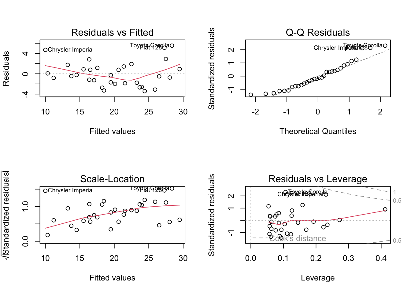
For practical diagnostics (residual analysis, heteroskedasticity testing, multicollinearity/VIF, and interaction effects), see Chapter 143.

Cramér, Harald. 1946. Mathematical Methods of Statistics. Princeton Mathematical Series 9. Princeton: Princeton University Press.

Rao, Calyampudi Radhakrishna. 1945. “Information and the Accuracy Attainable in the Estimation of Statistical Parameters.” Bulletin of the Calcutta Mathematical Society 37: 81–91.