143Hypothesis Testing with Linear Regression Models (from a Practical Point of View)
143.1 On the Relationship between Linear Regression Models and ANOVA
Let us reconsider the analysis that was presented in the discussion of the Two Way ANOVA model in Chapter 128. In the example we investigated the effect of two factors, i.e. Treatment with levels “A” and “B” and Gender with level “M” for males and “F” for females. The data was obtained within the framework of a well-designed, randomized experiment which implies that the underlying regression assumptions are most likely satisfied.
The MLRM for the Two Way ANOVA dataset can be formulated as follows:
where \(i\) is the index of the test subject (for \(i=1, 2, …, N\)), \(\alpha, \beta_1, \beta_2,\) and \(\gamma\) are regression parameters which need to be estimated by OLS, \(T_i\) is the variable Treatment (coded as a binary variable with \(T_i = 1\) when Treatment is equal to category “A”), \(G_i\) is Gender (coded as a binary variable with \(G_i = 1\) for males), and \(e_i\) is the prediction error of the model. The product \(T_iG_i\) is called the interaction between \(T_i\) and \(G_i\) and simply represents the situation where a male participant receives Treatment = “A” (because \(T_i G_i = 1\) if \(T_i = G_i = 1\)).
The main goal of the analysis presented below is to find out how MLRM differs from ANOVA. At the same time, we will discuss various Hypothesis Tests that can be performed based on the model parameters.
The OLS algorithm estimates the model parameters (\(\alpha, \beta_1, \beta_2,\) and \(\gamma\)) in such a way that the sum of squared residuals, i.e. \(\sum_{i=1}^{N} e_i^2\), is minimized. The analysis shows the regression model parameters based on the OLS estimation procedure. The variables have been given text-based names: \(T_i\) is labeled “AorB”, \(G_i\) is named “MorF”, and \(T_i G_i\) is labeled “Interaction”.
These results imply that the average response \(R_i = 3.05\) for all female participants receiving Treatment = “B” (because when \(T_i = G_i = 0\) then the regression equation reduces to \(R_i = 3.05 + e_i\)). Hence, the constant or intercept of the regression equation represents the baseline against which every other situation is compared. If we would have coded \(T_i\) or \(G_i\) differently, we would see a different value for the intercept. Hence, it is always important to know how the variables are coded in order to understand the results of the MLRM.
The average response for females receiving treatment “A” (instead of “B”) can be easily computed as follows:
On average \(e_i = 0\) (this is an underlying assumption), hence the difference of responses between females receiving “B” and “A” is \(3.05 - 1.45 = 1.6\) which is exactly the result which was presented in the output of the Two Way ANOVA analysis in Chapter 128.
Would it be possible to obtain the Two Way ANOVA effect which corresponds to “`B:M-A:M”? To find out, we need to compute the difference between two responses:
The response of males receiving “B” is \(R_i - e_i = 3.05 - 1.6 \times 0 - 2.13875 \times 1 + 1.24875 \times 0 = 0.91125\)
The response of males receiving “A” is \(R_i - e_i = 3.05 - 1.6 \times 1 - 2.13875 \times 1 + 1.24875 \times 1 = 0.56\)
Hence, the treatment effect for males is equal to \(0.91125 - 0.56 = 0.35125\) which is, again, exactly what we found in the ANOVA analysis.
Would it be possible to obtain the Two Way ANOVA effect which corresponds to “`B:M-B:F”? To find out, we need to compute the difference between:
The response of males receiving “B” is \(R_i - e_i = 3.05 - 1.6 \times 0 - 2.13875 \times 1 + 1.24875 \times 0 = 0.91125\)
The response of females receiving “B” is \(R_i - e_i = 3.05 - 1.6 \times 0 - 2.13875 \times 0 + 1.24875 \times 0 = 3.05\)
Hence, the gender effect of treatment “B” is equal to \(0.91125 - 3.05 = -2.13875\) which is, yet again, exactly the result from the ANOVA output.
Similarly, we could replicate each of the interactions between Treatment and Gender which was presented in the Two Way ANOVA table. How about the main effects of Treatment and Gender?
To compute the Treatment effect “B-A” we have to use the following four responses:
The “B” response for females is \(R_i - e_i = 3.05 -1.6 \times 0 - 2.13875 \times 0 + 1.24875 \times 0 = 3.05\)
The “B” response for males is \(R_i - e_i = 3.05 -1.6 \times 0 - 2.13875 \times 1 + 1.24875 \times 0 = 0.91125\)
The “A” response for females is \(R_i - e_i = 3.05 -1.6 \times 1 - 2.13875 \times 0 + 1.24875 \times 0 = 1.45\)
The “A” response for males is \(R_i - e_i = 3.05 -1.6 \times 1 - 2.13875 \times 1 + 1.24875 \times 1 = 0.56\)
Now we can compute the average “B” response as \((3.05 + 0.91125) / 2 = 1.980625\) because there are exactly the same number of females and males1. Similarly, the average “A” response is \((1.45 + 0.56) / 2 = 1.005\) which can be subtracted from the average “B” response to obtain “B-A”, i.e. \(1.980625 - 1.005 = 0.975625\). Again, we find exactly the same result as in Two Way ANOVA.
Of course, it is not a coincidence that both methods yield exactly the same results. Moreover, it is always possible to rewrite the regression equation in such a way that the main effects and interactions of the ANOVA results are obtained. The Regression and ANOVA models are, mathematically speaking, equivalent. Sometimes ANOVA is easier to use (e.g. when the factors or exogenous variables are categorical) and in other situations (e.g. when the exogenous variables are continuous) the regression models are more practical.
Note that the first Figure in the R module’s output shows the actual responses (full line) and the predicted averages (\(R_i - e_i\)) for each group (dots).
143.2 Testing Regression Model Assumptions
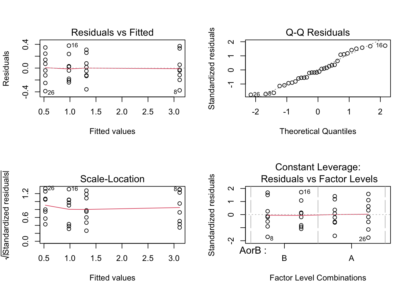
The differences between the predicted levels and actual responses are called residuals or prediction errors (\(e_i\)). These residuals are visualized in the Figure shown below and can be used to assess the underlying assumptions of the MLRM.
For instance, we can observe that the residuals are (more or less evenly) fluctuating around zero, i.e. the model does not systematically under- or overestimate the actual values, implying that the mean error is probably close to zero2. Even though the variances of each group are not equal (this is called heteroskedasticity), we already know that the effect of unequal variances can be mostly neglected when the groups have equal size. Furthermore, we can examine the distribution of the residuals, as is shown in the following analysis:
The residuals are fairly well represented by a Normal Distribution (i.e. there seems to be no serious deviation from normality). This visual check supports, but does not prove, the normal-error assumption used for exact small-sample t- and F-inference. Independence and homoskedasticity are separate assumptions that should also be assessed.
Of course, it is possible to use hypothesis testing to assess whether the data provide evidence consistent with the assumptions that the residual mean is zero, the variances are equal, and the residual distribution is approximately normal. As discussed in previous chapters, there are many procedures that can be helpful in this respect.
There are a couple of important statistics which are commonly reported in regression analysis and have the following interpretation:
The “Multiple R” statistic is simply the Pearson Correlation between the prediction of the model and the endogenous/dependent variable.
The “R-squared” is the square of the “Multiple R” statistic -- this is also called the “Determination Coefficient” and can be interpreted as the percentage of the variability of the endogenous variable that is explained by the MLRM. Obviously, the R-squared is a value between 0 and 1.
The “Adjusted R-squared” is an alternative measure for the “R-squared” which is corrected for the “Degrees of Freedom” of the model. It is useful for comparing OLS models with the same dependent variable, but it should be interpreted together with diagnostics and out-of-sample performance.
The F-test value and associated p-value are identical to the F-test of the corresponding ANOVA analysis. This can also be interpreted as the Hypothesis Test about R-squared: H\(_0: R^2 = 0\) versus H\(_A: R^2 > 0\). If the null is not rejected, we do not have sufficient evidence that the model explains variance beyond an intercept-only model.
The “Residual Standard Deviation” is simply the standard deviation of the prediction errors or, in other words, the expected prediction error that will occur when a single prediction is made based on the MLRM.
The “Sum of Squared Residuals” is the criterion which is minimized in the OLS procedure.
To test whether or not the model satisfies the equal variances assumption there are several types of so-called Heteroskedasticity Tests available. The R module in RFC features the Goldfeld-Quandt test (Goldfeld and Quandt 1965) which assumes that:
the observations are ordered group-wise (if any groups exist)
or the observations are ordered in chronological order (in case we are dealing with time series)
In our example, the observations are ordered group-wise as can be clearly observed in the first Figure of the regression output.
The Hypothesis of the Goldfeld-Quandt test, applied to the residuals \(e_i\), can be formulated as follows:
where \(j\) is the so-called breakpoint which divides the data in two parts, \(\sigma_{i \leq j}^2\) is the Variance of the first section, and \(\sigma_{i > j}^2\) is the Variance of the second section of the dataset under investigation.
Since we have information about many (sequential) Hypothesis Tests, each of which has a type I error, multiplicity should be handled with a pre-specified primary test or a formal correction (e.g., Holm, Bonferroni, or FDR). The output Table labeled “Meta Analysis of Goldfeld-Quandt test for Heteroskedasticity” is descriptive and should not be used as a standalone decision rule3.
143.3 Testing Regression Coefficients
The regression output lists all coefficients of the model, along with their statistics. This allows us to test each individual regression parameter, i.e. \(\alpha, \beta_1, \beta_2,\) and \(\gamma\) from the theoretical model formulation.
The Intercept \(\hat{\alpha} = 3.05\) has a Standard Deviation of \(0.1\) which implies that the t-Test for the intercept
The corresponding one-sided and two-sided p-values are very small which means that we reject the Null Hypothesis (implying that the intercept is not zero).
The treatment effect \(\hat{\beta_1} = -1.6\) has a Standard Deviation of \(0.1415\) which implies that the t-Test for this parameter
The corresponding one-sided and two-sided p-values are very small which means that we reject the Null Hypothesis (implying that \(\beta_1\) is not zero).
Similarly, we can draw the conclusion that \(\beta_2\) and \(\gamma\) are significantly different from zero (both have extremely small p-values).
The overall conclusion from the MLRM is that the main effects of the treatment and gender are both significant. In addition, the combined effect is significant as well, implying that gender interacts with the effect of the treatment (the treatment effect is not equal for males and females).
Note that in regression analysis the t-Test about the parameters, by convention, assumes that the Null value is equal to zero, i.e. \(\alpha_0 = \beta_{1,0} = \beta_{2,0} = \gamma_0 = 0\). Since this is not always appropriate it is fairly easy to build 95% confidence intervals based on the rough approximation that the lower and upper bounds are two Standard Deviations away from the parameter estimates. For instance, the approximate 95% interval of the estimated interaction parameter \(\hat{\gamma}\) is \([1.249 - 2 \times 0.2, 1.249 + 2 \times 0.2]\). With these confidence intervals it is easy to test the parameter against any Null value of interest.
143.4 Misspecification in Regression
In regression models it is almost always assumed that theoretical insights provide a “true” specification of the stochastic equation to be estimated. It is therefore obvious that if the (economic) theory is incomplete, the estimated parameters will (almost certainly) be biased. This bias which is introduced by “unobserved” (or forgotten) variables is called the “unobserved variables bias” (UVB).
Formally the UVB for a MLRM
\[
y = Xb + e
\]
can be illustrated, assuming the presence of unobserved variables \(Z\) with a corresponding parameter vector \(c\), by rewriting the OLS parameter equation as follows
\[
\begin{align*}b &= (X'X)^{-1}X'y \\&= (X'X)^{-1}X'(X\beta + Z c + e) \\&= \beta + (X'X)^{-1}X'Zc + (X'X)^{-1}X'e\end{align*}
\]
where \((X'X)^{-1}X'Zc\) are the so-called auxiliary regressions of the omitted variables on the exogenous variables \(X\) of the original (i.e. biased) equation.
It is also interesting to see that the residual variance is biased because
and since we assume that E\((e) = 0\), it follows that
\[
\text{E} (\hat{\sigma}^2) = \sigma^2 + \frac{\left[ \begin{matrix} \beta \\ c \end{matrix} \right]' \left[ \begin{matrix} X & Z \end{matrix} \right]' \Theta \left[ \begin{matrix} X & Z \end{matrix} \right] \left[ \begin{matrix} \beta \\ c \end{matrix} \right]}{n-k}
\]
such that E\((\hat{\sigma}^2) \geq \sigma^2\) (Q.E.D.).
A special kind of misspecification (i.e. one that is introduced by misspecified functional forms of the relationships between the dependent and independent variables) can (sometimes) be detected through the so-called Ramsey RESET specification test (Ramsey 1969). This test is based on a test-equation in which the original specification is expanded with powers of the interpolation fit (powers of 2, 3, etc.). The number of terms to be added is user-defined and the corresponding parameters can be tested with an ordinary F-test. If the Null Hypothesis of this F-test is rejected, it is concluded that the added terms contribute to the prediction of the endogenous variable, which automatically implies that the original equation is most likely misspecified.
The implementation of the Ramsey RESET test in RFC uses three test equations, each of which is based on different terms: powers (2 and 3) of the fitted values, powers (2 and 3) of the actual regressors, and powers (2 and 3) of the principal components. For each of these test equations the F-test is computed.
143.5 Multicollinearity in Regression
143.5.1 Theoretical Aspects of Multicollinearity
As explained in Section 135.1.8, the parameters from estimating repeated SLRMs are identical to the results of a single MLRM where all parameters are computed simultaneously, provided the exogenous variables are orthogonal (independent). However, when two or more exogenous variables are mutually correlated, they are not independent (which is commonly referred to as multicollinearity).
Consider the simple case of two vectors \(x_1\) and \(x_2\) which are taken from the set of \(n\) exogenous variables. These vectors are called multicollinear if
which means that both vectors are perfectly correlated (linearly dependent).
In this case it is not possible to make a distinction between the effects of \(x_1\) and \(x_2\) on the endogenous variable because they are both indistinguishable (we call this perfect multicollinearity). Mathematically speaking, the OLS parameters cannot be computed because the OLS estimator \(b = (X'X)^{-1} X'y\) contains a singular matrix \((X'X)\) which cannot be inverted. In this sense, it is a strict requirement that the \(X'X\) matrix is non-singular.
Now we consider the (more realistic) case of exogenous variables which are mutually correlated (but without being perfectly, linearly dependent). Denote \(X'X\) as a square \(K*K\) matrix \(A\) and consider an orthogonal \(K*K\) matrix \(G\) with columns \(g_1, g_2, …, g_K\). The columns \(g_i\) are assumed to be the eigenvectors (corresponding to different latent roots) of the square matrix \(A\).
Since \(GG' = I\) we can write the MLRM as
\[
y = (XG)(G'\beta) + e = Z \delta + e
\]
where the columns of \(Z\) are called “principal components” which are (by definition) orthogonal with respect to each other and have a length which is equal to their eigenvalue.
Since \(X'X\) (equivalently \(Z'Z\)) is symmetric and positive semi definite, it follows that the eigenvalues are real and non-negative. In addition, it can be easily verified that
from which it can be deduced that the variance of \(\hat{\delta}_j\) becomes large when the eigenvalue is small (smaller than 1). In the extreme case where the eigenvalue converges to zero, the variance becomes extremely large (tending towards infinity in the case of perfect multicollinearity).
How does this result affect the variance of the parameters in the original MLRM? To answer this question, we need to consider the fact that
\[
G'\hat{\beta} = \hat{\delta} \Rightarrow \hat{\beta} = G \hat{\delta}
\]
which does not necessarily imply that low lambda values yield high variances (this also depends on the other parameters in the regression). Therefore, in general, low lambda values do not always imply that the variances are inflated (but it is possible).
143.5.2 Detection of Multicollinearity
From the previous section we can conclude that strong linear associations between exogenous variables are not always catastrophic. Hence the proposed multicollinearity diagnostics should be used with care.
143.5.2.1 Correlation Matrix
The correlation matrix can be used as a preliminary screening tool for linear associations among exogenous variables. However, pairwise correlations alone are not a reliable diagnostic for harmful multicollinearity; use established diagnostics such as VIF, condition indices/eigenvalues, and variance-decomposition proportions for inference.
143.5.2.2 High R-squared and low t-Statistics
When the determination coefficient (\(R^2\)) is reasonably high while all or most regression parameters have low t-Statistics (i.e. they are not significantly different from zero), this may be viewed as a symptom of harmful multicollinearity. As explained before, multicollinearity manifests itself by inflating the variances (which decreases the t-Statistics of the parameters) -- it does not, however, affect the ability of the model to explain the endogenous variable (hence the \(R^2\) might still be reasonably high).
143.5.2.3 High R-squared and low partial correlation between an exogenous variable and the dependent variable
Again, low partial correlations between exogenous and endogenous variables, is symptomatic for multicollinearity. In particular, if the partial correlation is much lower than the ordinary Pearson correlation, it can be concluded that the exogenous variable does not contribute more than what is already explained by the other variables.
143.5.2.4 Variance Inflation Factors
It is obvious that multicollinearity may exist when the exogenous variables have an impact on each other. This can be measured by the R-squared of the auxiliary regression which explains any chosen exogenous variable based on all other \(K - 1\) variables (including a constant term). The higher the R-squared of such an auxiliary regression, the higher the degree of multicollinearity.
The respective F-statistic may be calculated as follows
The same information can be expressed in terms of the so-called Variance Inflation Factors:
\[
\text{VIF}_i = \frac{1}{(1-R_i^2)}
\]
where \(R_i^2\) is the determination coefficient of the auxiliary regression which explains \(x_i\). As the name indicates, VIF measures the factor by which the parameter’s variance is multiplied (inflated) as compared to an orthogonal regression (where all exogenous variables are independent).
143.5.3 Remedies for Multicollinearity
143.5.3.1 Drop spurious exogenous variables
Suppose we were interested in the estimation of the model
where \(G_t, I_t, H_t, L_t\), and \(A_t\) are exogenous variables.
In addition, suppose that harmful multicollinearity would have been discovered between the first three (\(G_t, I_t\), and \(H_t\)) and the last two variables (\(L_t\) and \(A_t\)). In this scenario we may select one representative of each group (e.g. \(G_t\) and \(L_t\)) while all the other exogenous variables are dropped (because they do not contain any additional information which is not already present in either \(G_t\) or \(L_t\)).
143.5.3.2 Principal Components
As explained before, \(X'X\) can be diagonalized and written in terms of eigenvectors and eigenvalues. Accordingly, the linear model can be written in terms of its principal components. The first principal component can intuitively be interpreted as the summary of all exogenous variables by one column vector which explains as much of X as possible. The remaining information is contained in the second principal component and so on … It is, however, important to note that the principal components are orthogonal and therefore cannot be multicollinear.
Suppose we would have computed the principal components for the model of the previous section. Also assume that the principal components (PC) contain (in descending order) 90%, 5%, 4%, … of the total variance of the exogenous variables. In such circumstances we would retain the first three PCs in our regression model since they account for 99% of the variance of \(X\).
When having three PCs in a regression model, this means that there are three important groups of variables (within the set of X) which are explaining the endogenous variable. Cross correlations between the exogenous variables and the PCs should reveal which variables may be associated with different factors (this is necessary for interpretation purposes).
Now suppose that this regression would result in only the first PC’s parameter to be significantly different from zero. In this case our model would reduce to a simple regression. In this particular case we can look at the correlations between the exogenous variables and the first PC to determine which of the original variables is important. However, if more than just one PC has a significant regression parameter, it is much more difficult to assess the importance of each of the original variables.
Therefore, in such circumstances, it could be better to compute the PC for both subgroups that we have detected before. We may present the X matrix as follows
and compute the PC for S and T separately. This process will probably result in at least one significant PC-parameter per subgroup in a multiple regression -- therefore, it is rather easy to interpret the model. Note, however, that in this case there is no reason to assume that the first PC of S and the first PC or T are not multicollinear. More importantly, since both PCs have been computed separately, and since our splitting of the variables into two subgroups, might have been wrong, there is no guarantee that the PCs are optimal in a global sense (for the complete regression model).
Due to these problems, the PC approach has not been implemented in RFC. Instead, there is an alternative approach (i.e. Partial Least Squares) which is, statistically speaking, superior because it does not suffer from these shortcomings and provides easily interpretable results at the same time.
143.6 How to Code Multiple Regression in R
Even though the Multiple Regression module can be found on the public website (https://compute.wessa.net/rwasp_multipleregression.wasp) and in RFC (under the Models / Manual Model Building menu), it is easy to reproduce the ANOVA-equivalent regression analysis locally with a compact script:
set.seed(123)# Balanced 2x2 design (Treatment x Gender), 8 observations per celln_cell <-8AorB <-rep(c('B', 'A'), each =2* n_cell)MorF <-rep(rep(c('F', 'M'), each = n_cell), times =2)# Cell means chosen to match the chapter discussionmu <-ifelse(AorB =='B'& MorF =='F', 3.05,ifelse(AorB =='A'& MorF =='F', 1.45,ifelse(AorB =='B'& MorF =='M', 0.91125, 0.56)))R <- mu +rnorm(length(mu), mean =0, sd =0.25)df <-data.frame(R = R,AorB =factor(AorB, levels =c('B', 'A')),MorF =factor(MorF, levels =c('F', 'M')))# MLRM equivalent to two-way ANOVA with interactionfit <-lm(R ~ AorB * MorF, data = df)summary(fit)# Same model in ANOVA formanova(fit)
Call:
lm(formula = R ~ AorB * MorF, data = df)

Residuals:
     Min       1Q   Median       3Q      Max
-0.38813 -0.14488 -0.03331  0.16449  0.37817

Coefficients:
            Estimate Std. Error t value Pr(>|t|)
(Intercept)  3.10871    0.08313  37.395  < 2e-16 ***
AorBA       -1.79249    0.11756 -15.247 4.34e-15 ***
MorFM       -2.12890    0.11756 -18.108  < 2e-16 ***
AorBA:MorFM  1.33913    0.16626   8.054 9.04e-09 ***
---
Signif. codes:  0 '***' 0.001 '**' 0.01 '*' 0.05 '.' 0.1 ' ' 1

Residual standard error: 0.2351 on 28 degrees of freedom
Multiple R-squared:  0.952, Adjusted R-squared:  0.9469
F-statistic: 185.2 on 3 and 28 DF,  p-value: < 2.2e-16

Analysis of Variance Table

Response: R
          Df  Sum Sq Mean Sq F value    Pr(>F)
AorB       1 10.0876 10.0876 182.464 8.690e-14 ***
MorF       1 17.0373 17.0373 308.168 < 2.2e-16 ***
AorB:MorF  1  3.5866  3.5866  64.873 9.039e-09 ***
Residuals 28  1.5480  0.0553
---
Signif. codes:  0 '***' 0.001 '**' 0.01 '*' 0.05 '.' 0.1 ' ' 1
Code
par(mfrow =c(2, 2))plot(fit)par(mfrow =c(1, 1))
Figure 143.1: Residual diagnostics for the ANOVA-equivalent MLRM
# Goldfeld-Quandt test (ordered by fitted values)if (requireNamespace('lmtest', quietly =TRUE)) {print(lmtest::gqtest(fit, order.by =fitted(fit), alternative ='two.sided'))}# Variance inflation factorsif (requireNamespace('car', quietly =TRUE)) {print(car::vif(fit))}
    Goldfeld-Quandt test

data:  fit
GQ = 1.0096, df1 = 12, df2 = 12, p-value = 0.9871
alternative hypothesis: variance changes from segment 1 to 2

     AorB      MorF AorB:MorF
        2         2         3
This compact workflow focuses on the chapter’s core objective: linking two-way ANOVA and MLRM, then checking residual assumptions and coefficient inference.
Goldfeld, Stephen M., and Richard E. Quandt. 1965. “Some Tests for Homoscedasticity.”Journal of the American Statistical Association 60 (310): 539–47. https://doi.org/10.1080/01621459.1965.10480811.
Ramsey, J. B. 1969. “Tests for Specification Errors in Classical Linear Least-Squares Regression Analysis.”Journal of the Royal Statistical Society: Series B (Methodological) 31 (2): 350–71. https://doi.org/10.1111/j.2517-6161.1969.tb00796.x.
If the number of females and males were unequal, we would have to use a weighted mean instead.↩︎
The summary statistics are shown at the bottom of the output and confirm that the Arithmetic Mean is equal to 0.00000 (rounded to 5 decimal places).↩︎
Use a formal multiple-testing correction (e.g., Holm, Bonferroni, or FDR) when combining evidence from several tests.↩︎