• Descriptive
    • Moments
    • Concentration
    • Central Tendency
    • Variability
    • Stem-and-Leaf Plot
    • Histogram & Frequency Table
    • Data Quality Forensics
    • Conditional EDA
    • Quantiles
    • Kernel Density Estimation
    • Normal QQ Plot
    • Bootstrap Plot

    • Multivariate Descriptive Statistics
  • Distributions
    • Binomial Probabilities
    • Geometric Probabilities
    • Negative Binomial Probabilities
    • Hypergeometric Probabilities
    • Multinomial Probabilities
    • Dirichlet
    • Poisson Probabilities

    • Exponential
    • Gamma
    • Erlang
    • Weibull
    • Rayleigh
    • Maxwell-Boltzmann
    • Lognormal
    • Pareto
    • Inverse Gamma
    • Inverse Chi-Square

    • Beta
    • Power
    • Beta Prime (Inv. Beta)
    • Triangular

    • Normal (area)
    • Logistic
    • Laplace
    • Cauchy (standard)
    • Cauchy (location-scale)
    • Gumbel
    • Fréchet
    • Generalized Extreme Value

    • Normal RNG
    • ML Fitting
    • Tukey Lambda PPCC
    • Box-Cox Normality Plot
    • Noncentral t
    • Noncentral F
    • Sample Correlation r

    • Empirical Tests
  • Hypotheses
    • Theoretical Aspects of Hypothesis Testing
    • Bayesian Inference
    • Minimum Sample Size

    • Empirical Tests
    • Multivariate (pair-wise) Testing
  • Models
    • Manual Model Building
    • Guided Model Building
  • Time Series
    • Time Series Plot
    • Decomposition
    • Exponential Smoothing

    • Blocked Bootstrap Plot
    • Mean Plot
    • (P)ACF
    • VRM
    • Standard Deviation-Mean Plot
    • Spectral Analysis
    • ARIMA

    • Cross Correlation Function
    • Granger Causality
  1. Descriptive Statistics & Exploratory Data Analysis
  2. 60  ROC Analysis
  • Preface
  • Getting Started
    • 1  Introduction
    • 2  Why Do We Need Innovative Technology?
    • 3  Basic Definitions
    • 4  The Big Picture: Why We Analyze Data
  • Introduction to Probability
    • 5  Definitions of Probability
    • 6  Jeffreys’ axiom system
    • 7  Bayes’ Theorem
    • 8  Sensitivity and Specificity
    • 9  Naive Bayes Classifier
    • 10  Law of Large Numbers

    • 11  Problems
  • Probability Distributions
    • 12  Bernoulli Distribution
    • 13  Binomial Distribution
    • 14  Geometric Distribution
    • 15  Negative Binomial Distribution
    • 16  Hypergeometric Distribution
    • 17  Multinomial Distribution
    • 18  Poisson Distribution

    • 19  Uniform Distribution (Rectangular Distribution)
    • 20  Normal Distribution (Gaussian Distribution)
    • 21  Gaussian Naive Bayes Classifier
    • 22  Chi Distribution
    • 23  Chi-squared Distribution (1 parameter)
    • 24  Chi-squared Distribution (2 parameters)
    • 25  Student t-Distribution
    • 26  Fisher F-Distribution
    • 27  Exponential Distribution
    • 28  Lognormal Distribution
    • 29  Gamma Distribution
    • 30  Beta Distribution
    • 31  Weibull Distribution
    • 32  Pareto Distribution
    • 33  Inverse Gamma Distribution
    • 34  Rayleigh Distribution
    • 35  Erlang Distribution
    • 36  Logistic Distribution
    • 37  Laplace Distribution
    • 38  Gumbel Distribution
    • 39  Cauchy Distribution
    • 40  Triangular Distribution
    • 41  Power Distribution
    • 42  Beta Prime Distribution
    • 43  Sample Correlation Distribution
    • 44  Dirichlet Distribution
    • 45  Generalized Extreme Value (GEV) Distribution
    • 46  Frechet Distribution
    • 47  Noncentral t Distribution
    • 48  Noncentral F Distribution
    • 49  Inverse Chi-Squared Distribution
    • 50  Maxwell-Boltzmann Distribution
    • 51  Distribution Relationship Map

    • 52  Problems
  • Descriptive Statistics & Exploratory Data Analysis
    • 53  Types of Data
    • 54  Datasheets

    • 55  Frequency Plot (Bar Plot)
    • 56  Frequency Table
    • 57  Contingency Table
    • 58  Binomial Classification Metrics
    • 59  Confusion Matrix
    • 60  ROC Analysis

    • 61  Stem-and-Leaf Plot
    • 62  Histogram
    • 63  Data Quality Forensics
    • 64  Quantiles
    • 65  Central Tendency
    • 66  Variability
    • 67  Skewness & Kurtosis
    • 68  Concentration
    • 69  Notched Boxplot
    • 70  Scatterplot
    • 71  Pearson Correlation
    • 72  Rank Correlation
    • 73  Partial Pearson Correlation
    • 74  Simple Linear Regression
    • 75  Moments
    • 76  Quantile-Quantile Plot (QQ Plot)
    • 77  Normal Probability Plot
    • 78  Probability Plot Correlation Coefficient Plot (PPCC Plot)
    • 79  Box-Cox Normality Plot
    • 80  Kernel Density Estimation
    • 81  Bivariate Kernel Density Plot
    • 82  Conditional EDA: Panel Diagnostics
    • 83  Bootstrap Plot (Central Tendency)
    • 84  Survey Scores Rank Order Comparison
    • 85  Cronbach Alpha

    • 86  Equi-distant Time Series
    • 87  Time Series Plot (Run Sequence Plot)
    • 88  Mean Plot
    • 89  Blocked Bootstrap Plot (Central Tendency)
    • 90  Standard Deviation-Mean Plot
    • 91  Variance Reduction Matrix
    • 92  (Partial) Autocorrelation Function
    • 93  Periodogram & Cumulative Periodogram

    • 94  Problems
  • Hypothesis Testing
    • 95  Normal Distributions revisited
    • 96  The Population
    • 97  The Sample
    • 98  The One-Sided Hypothesis Test
    • 99  The Two-Sided Hypothesis Test
    • 100  When to use a one-sided or two-sided test?
    • 101  What if \(\sigma\) is unknown?
    • 102  The Central Limit Theorem (revisited)
    • 103  Statistical Test of the Population Mean with known Variance
    • 104  Statistical Test of the Population Mean with unknown Variance
    • 105  Statistical Test of the Variance
    • 106  Statistical Test of the Population Proportion
    • 107  Statistical Test of the Standard Deviation \(\sigma\)
    • 108  Statistical Test of the difference between Means -- Independent/Unpaired Samples
    • 109  Statistical Test of the difference between Means -- Dependent/Paired Samples
    • 110  Statistical Test of the difference between Variances -- Independent/Unpaired Samples

    • 111  Hypothesis Testing for Research Purposes
    • 112  Decision Thresholds, Alpha, and Confidence Levels
    • 113  Bayesian Inference for Decision-Making
    • 114  One Sample t-Test
    • 115  Skewness & Kurtosis Tests
    • 116  Paired Two Sample t-Test
    • 117  Wilcoxon Signed-Rank Test
    • 118  Unpaired Two Sample t-Test
    • 119  Unpaired Two Sample Welch Test
    • 120  Two One-Sided Tests (TOST) for Equivalence
    • 121  Mann-Whitney U test (Wilcoxon Rank-Sum Test)
    • 122  Bayesian Two Sample Test
    • 123  Median Test based on Notched Boxplots
    • 124  Chi-Squared Tests for Count Data
    • 125  Kolmogorov-Smirnov Test
    • 126  One Way Analysis of Variance (1-way ANOVA)
    • 127  Kruskal-Wallis Test
    • 128  Two Way Analysis of Variance (2-way ANOVA)
    • 129  Repeated Measures ANOVA
    • 130  Friedman Test
    • 131  Testing Correlations
    • 132  A Note on Causality

    • 133  Problems
  • Regression Models
    • 134  Simple Linear Regression Model (SLRM)
    • 135  Multiple Linear Regression Model (MLRM)
    • 136  Logistic Regression
    • 137  Generalized Linear Models
    • 138  Multinomial and Ordinal Logistic Regression
    • 139  Cox Proportional Hazards Regression
    • 140  Conditional Inference Trees
    • 141  Leaf Diagnostics for Conditional Inference Trees
    • 142  Conditional Random Forests
    • 143  Hypothesis Testing with Linear Regression Models (from a Practical Point of View)

    • 144  Problems
  • Introduction to Time Series Analysis
    • 145  Case: the Market of Health and Personal Care Products
    • 146  Decomposition of Time Series
    • 147  Ad hoc Forecasting of Time Series
  • Box-Jenkins Analysis
    • 148  Introduction to Box-Jenkins Analysis
    • 149  Theoretical Concepts
    • 150  Stationarity
    • 151  Identifying ARMA parameters
    • 152  Estimating ARMA Parameters and Residual Diagnostics
    • 153  Forecasting with ARIMA models
    • 154  Intervention Analysis
    • 155  Cross-Correlation Function
    • 156  Transfer Function Noise Models
    • 157  General-to-Specific Modeling
  • Model Building Strategies
    • 158  Introduction to Model Building Strategies
    • 159  Manual Model Building
    • 160  Model Validation
    • 161  Regularization Methods
    • 162  Hyperparameter Optimization Strategies
    • 163  Guided Model Building in Practice
    • 164  Diagnostics, Revision, and Guided Forecasting
    • 165  Leakage, Target Encoding, and Robust Regression
  • References
  • Appendices
    • Appendices
    • A  Method Selection Guide
    • B  Presentations and Teaching Materials
    • C  R Language Concepts for Statistical Computing
    • D  Matrix Algebra
    • E  Standard Normal Table (Gaussian Table)
    • F  Critical values of Student’s \(t\) distribution with \(\nu\) degrees of freedom
    • G  Upper-tail critical values of the \(\chi^2\)-distribution with \(\nu\) degrees of freedom
    • H  Lower-tail critical values of the \(\chi^2\)-distribution with \(\nu\) degrees of freedom

Table of contents

  • 60.1 Definition
  • 60.2 The Classification Threshold
    • 60.2.1 The Trade-off
    • 60.2.2 Example: Fraud Detection
  • 60.3 Constructing the ROC Curve
    • 60.3.1 Interpreting the ROC Curve
    • 60.3.2 R Code for ROC Curve Construction
  • 60.4 Area Under the Curve (AUC)
    • 60.4.1 Definition
    • 60.4.2 Interpretation
    • 60.4.3 Connection to the Mann-Whitney U Statistic
    • 60.4.4 Computing AUC in R
  • 60.5 The Pay-off Matrix and Optimal Threshold Selection
    • 60.5.1 The Pay-off Matrix
    • 60.5.2 Example: Fraud Detection Pay-offs
    • 60.5.3 Expected Cost at a Given Threshold
    • 60.5.4 Threshold Selection Methods
  • 60.6 R Module
    • 60.6.1 Public website
    • 60.6.2 RFC
  • 60.7 Example
  • 60.8 ROC Analysis and p-values
  • 60.9 Pros & Cons
    • 60.9.1 Pros
    • 60.9.2 Cons
  • 60.10 Task
  1. Descriptive Statistics & Exploratory Data Analysis
  2. 60  ROC Analysis

60  ROC Analysis

60.1 Definition

ROC stands for Receiver Operating Characteristic. It is a method that evaluates the performance of binary classifiers across all possible classification thresholds. The method was originally developed in signal detection theory (Green and Swets 1966) (during World War II) for radar operators who needed to distinguish enemy aircraft from noise.

In previous chapters, we introduced the Confusion Matrix (Chapter 59) and various classification metrics including Sensitivity, Specificity, and the concepts of True Positives, True Negatives, False Positives, and False Negatives. These metrics were computed for a single, fixed classification threshold. ROC analysis extends this by examining how classifier performance changes as the threshold varies.

60.2 The Classification Threshold

Binary classifiers such as the Naive Bayes Classifier (Chapter 9) do not directly produce binary predictions. Instead, they produce probability scores — estimates of the probability that each observation belongs to the positive class. To convert these probabilities into binary predictions, we must choose a classification threshold.

The classification rule is simple: if the predicted probability P(positive) is greater than or equal to the threshold, we predict positive; otherwise, we predict negative.

\[ \text{Prediction} = \begin{cases} \text{Positive} & \text{if } P(\text{positive}) \geq \text{threshold} \\ \text{Negative} & \text{if } P(\text{positive}) < \text{threshold} \end{cases} \]

60.2.1 The Trade-off

The choice of threshold directly affects the balance between Sensitivity and Specificity:

  • Lowering the threshold makes the classifier more likely to predict positive. This increases Sensitivity (we catch more true positives) but decreases Specificity (we also generate more false positives).

  • Raising the threshold makes the classifier more conservative. This increases Specificity (fewer false alarms) but decreases Sensitivity (we miss more true positives).

There is no threshold that simultaneously maximizes both Sensitivity and Specificity. The choice of threshold depends on the relative costs of different types of errors.

This threshold-choice problem is an example of a more general idea used throughout this handbook: decision thresholds depend on purpose. In ROC analysis, we choose a classification threshold based on the trade-off between false positives and false negatives (and their costs). In hypothesis testing, the same logic reappears when choosing a significance threshold \(\alpha\). The general framework is discussed in Chapter 112.

60.2.2 Example: Fraud Detection

Continuing the fraud detection example from Chapter 58 and Chapter 59, suppose our Naive Bayes classifier produces the following probability scores for seven transactions:

Table 60.1: Fraud Probability Scores
Transaction Actual Fraud P(Fraud)
1 No 0.62
2 Yes 0.81
3 No 0.15
4 No 0.23
5 Yes 0.38
6 No 0.09
7 Yes 0.44

At threshold = 0.50:

  • Transactions 1 and 2 are predicted as fraud (P ≥ 0.50)
  • Transaction 2 is correctly identified (TP = 1), but transaction 1 is a false alarm (FP = 1)
  • Transactions 5 and 7 are missed (FN = 2)

At threshold = 0.35:

  • Transactions 1, 2, 5, and 7 are predicted as fraud
  • We catch more fraud (TP = 3) but still have a false alarm (FP = 1)
  • Transactions 5 (P = 0.38) and 7 (P = 0.44) are now additionally correctly identified

The confusion matrix changes with every threshold choice, and so do all the derived metrics.

60.3 Constructing the ROC Curve

The ROC curve visualizes classifier performance across all possible thresholds. It is constructed as follows:

  1. For each possible threshold value (from 0 to 1):

    • Classify all observations using that threshold
    • Compute the Confusion Matrix
    • Calculate the True Positive Rate (TPR = Sensitivity)
    • Calculate the False Positive Rate (FPR = 1 − Specificity)
  2. Plot each (FPR, TPR) pair as a point

  3. Connect the points to form the ROC curve

60.3.1 Interpreting the ROC Curve

The ROC curve is plotted with:

  • X-axis: False Positive Rate (FPR) ranging from 0 to 1
  • Y-axis: True Positive Rate (TPR) ranging from 0 to 1

Key reference points:

  • Bottom-left corner (0, 0): Threshold = 1.0. No positive predictions are made, so TPR = 0 and FPR = 0.
  • Top-right corner (1, 1): Threshold = 0.0. All predictions are positive, so TPR = 1 and FPR = 1.
  • Top-left corner (0, 1): Perfect classification. All positives are correctly identified (TPR = 1) with no false alarms (FPR = 0).
  • Diagonal line: Random guessing. A classifier with no discriminative ability produces points along the diagonal.

A good classifier produces an ROC curve that bows toward the top-left corner, staying well above the diagonal.

60.3.2 R Code for ROC Curve Construction

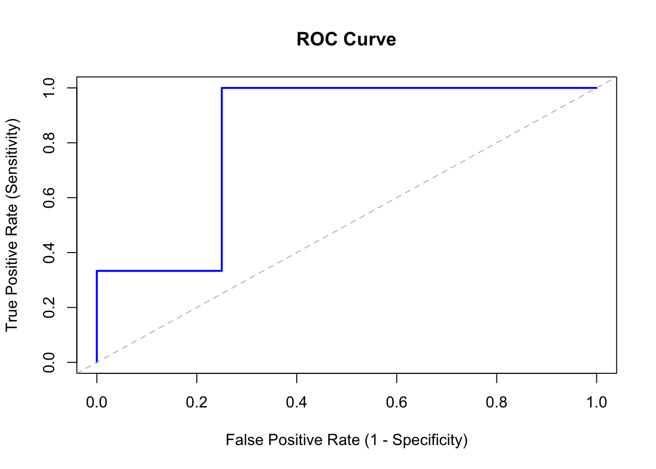
The following code demonstrates how to construct an ROC curve from scratch:

# Example data: predicted probabilities and actual outcomes
predicted_prob <- c(0.62, 0.81, 0.15, 0.23, 0.38, 0.09, 0.44)
actual <- c(0, 1, 0, 0, 1, 0, 1)  # 1 = Fraud, 0 = No Fraud

# Function to compute TPR and FPR at a given threshold
compute_rates <- function(threshold, probs, actuals) {
  predictions <- as.integer(probs >= threshold)
  TP <- sum(predictions == 1 & actuals == 1)
  FP <- sum(predictions == 1 & actuals == 0)
  TN <- sum(predictions == 0 & actuals == 0)
  FN <- sum(predictions == 0 & actuals == 1)
  TPR <- TP / (TP + FN)  # Sensitivity
  FPR <- FP / (FP + TN)  # 1 - Specificity
  return(c(FPR = FPR, TPR = TPR))
}

# Compute ROC curve points
thresholds <- seq(0, 1, by = 0.01)
roc_points <- t(sapply(thresholds, compute_rates,
                        probs = predicted_prob,
                        actuals = actual))

# Plot ROC curve
plot(roc_points[, "FPR"], roc_points[, "TPR"],
     type = "l", lwd = 2, col = "blue",
     xlab = "False Positive Rate (1 - Specificity)",
     ylab = "True Positive Rate (Sensitivity)",
     main = "ROC Curve",
     xlim = c(0, 1), ylim = c(0, 1))
abline(a = 0, b = 1, lty = 2, col = "gray")  # Diagonal reference line

For larger datasets and more sophisticated analysis, the pROC package provides comprehensive ROC functionality:

library(pROC)
roc_obj <- roc(actual, predicted_prob)
plot(roc_obj, main = "ROC Curve (pROC package)")

60.4 Area Under the Curve (AUC)

The Area Under the ROC Curve (AUC) provides a single summary measure of classifier performance across all thresholds.

60.4.1 Definition

The AUC has an intuitive probabilistic interpretation (Hanley and McNeil 1982): it represents the probability that the classifier will rank a randomly chosen positive instance higher than a randomly chosen negative instance.

\[ \text{AUC} = P(\text{score}_{positive} > \text{score}_{negative}) \]

60.4.2 Interpretation

Table 60.2: AUC Interpretation Guidelines (Hosmer and Lemeshow 2000)
AUC Value Interpretation
0.5 No discriminative ability (random guessing)
0.5 – 0.6 Poor
0.6 – 0.7 Moderate
0.7 – 0.8 Acceptable
0.8 – 0.9 Good
0.9 – 1.0 Excellent
1.0 Perfect discrimination

An AUC of 0.5 indicates the classifier performs no better than random coin flipping. An AUC below 0.5 suggests the classifier is systematically wrong (predictions are inverted).

60.4.3 Connection to the Mann-Whitney U Statistic

The AUC is mathematically equivalent to the Mann-Whitney U statistic (normalized to [0, 1]), which was introduced in Chapter 121. This connection provides a non-parametric way to test whether a classifier’s AUC is significantly greater than 0.5.

60.4.4 Computing AUC in R

# Manual AUC computation using the trapezoidal rule
compute_auc <- function(fpr, tpr) {
  # Sort by FPR
  ord <- order(fpr)
  fpr <- fpr[ord]
  tpr <- tpr[ord]
  # Trapezoidal integration
  sum(diff(fpr) * (head(tpr, -1) + tail(tpr, -1)) / 2)
}

auc_value <- compute_auc(roc_points[, "FPR"], roc_points[, "TPR"])
cat("AUC:", round(auc_value, 3), "\n")
AUC: 0.792 

60.5 The Pay-off Matrix and Optimal Threshold Selection

While AUC summarizes overall discrimination ability, it does not tell us which threshold to use in practice. The optimal threshold depends on the costs and benefits of different classification outcomes.

60.5.1 The Pay-off Matrix

The pay-off matrix assigns economic values to each cell of the Confusion Matrix:

Table 60.3: The Pay-off Matrix
Actual Positive Actual Negative
Predict Positive Benefit(TP) or 0 Cost(FP)
Predict Negative Cost(FN) Benefit(TN) or 0

In many applications, we define the costs relative to correct classifications (which have zero cost), so the pay-off matrix simplifies to specifying:

  • Cost(FP): The cost of a false positive (false alarm)
  • Cost(FN): The cost of a false negative (missed detection)

60.5.2 Example: Fraud Detection Pay-offs

In fraud detection:

  • Cost(FN): A missed fraud means stolen funds must be reimbursed. Suppose this averages €500 per incident.
  • Cost(FP): A false alarm means a legitimate transaction is blocked, causing customer inconvenience and potential lost business. Suppose this costs €10 per incident.

The asymmetry is clear: missing a fraud is 50 times more costly than a false alarm. This should influence our threshold choice — we should be willing to accept more false alarms to catch more fraud.

60.5.3 Expected Cost at a Given Threshold

For a given threshold, the expected cost per classification is:

\[ \text{Expected Cost} = \text{Cost(FP)} \times \text{FPR} \times P(\text{Negative}) + \text{Cost(FN)} \times \text{FNR} \times P(\text{Positive}) \]

where:

  • FPR = False Positive Rate
  • FNR = False Negative Rate = 1 − TPR
  • P(Positive) = Prevalence of the positive class
  • P(Negative) = 1 − Prevalence

The optimal threshold minimizes the expected cost (or equivalently, maximizes expected benefit).

60.5.4 Threshold Selection Methods

60.5.4.1 Youden’s Index

When costs are assumed equal (or unknown), Youden’s Index (Youden 1950) provides a simple criterion:

\[ J = \text{Sensitivity} + \text{Specificity} - 1 = \text{TPR} - \text{FPR} \]

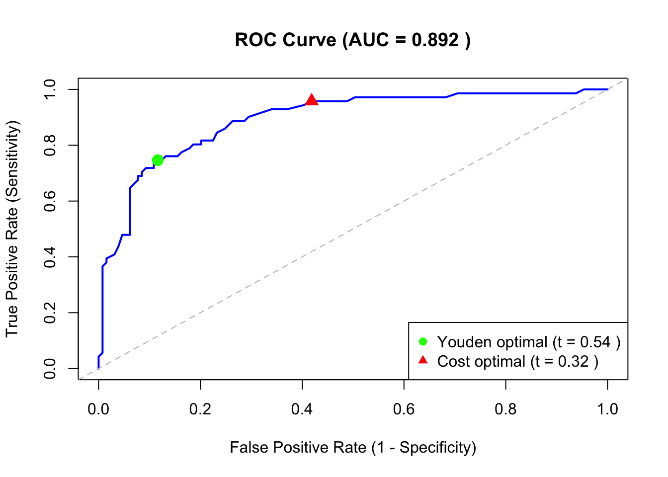
The optimal threshold maximizes \(J\). This is equivalent to finding the point on the ROC curve farthest from the diagonal. Note that Youden’s Index is identical to the Informedness metric introduced in Chapter 59.

60.5.4.2 Cost-based Optimization

When costs are known, the optimal threshold minimizes expected cost:

# Define costs
cost_FP <- 10    # Cost of false positive
cost_FN <- 500   # Cost of false negative
prevalence <- mean(actual)  # P(Positive)

# Compute expected cost at each threshold
compute_expected_cost <- function(fpr, tpr, cost_FP, cost_FN, prevalence) {
  fnr <- 1 - tpr
  cost_FP * fpr * (1 - prevalence) + cost_FN * fnr * prevalence
}

expected_costs <- mapply(compute_expected_cost,
                          fpr = roc_points[, "FPR"],
                          tpr = roc_points[, "TPR"],
                          MoreArgs = list(cost_FP = cost_FP,
                                          cost_FN = cost_FN,
                                          prevalence = prevalence))

optimal_idx <- which.min(expected_costs)
optimal_threshold <- thresholds[optimal_idx]
cat("Optimal threshold (cost-based):", optimal_threshold, "\n")
cat("Expected cost at optimal threshold:", round(expected_costs[optimal_idx], 2), "\n")
Optimal threshold (cost-based): 0.24 
Expected cost at optimal threshold: 1.43 

60.5.4.3 Domain Constraints

In some applications, hard constraints may apply:

  • Medical screening: “Sensitivity must be at least 95%”
  • Security systems: “Specificity must be at least 99%”

In such cases, the optimal threshold is the one that satisfies the constraint while optimizing the secondary metric.

60.6 R Module

60.6.1 Public website

ROC Analysis is available on the public website:

  • https://compute.wessa.net/roc.wasp

60.6.2 RFC

The ROC Analysis module is available in RFC under the menu “Models / Manual model building”.

60.7 Example

The following example demonstrates ROC analysis using simulated classifier output:

# Simulate a larger dataset
set.seed(42)
n <- 200
actual_large <- rbinom(n, 1, 0.3)  # 30% positive rate

# Simulate classifier scores (higher for positives)
scores_large <- ifelse(actual_large == 1,
                        rbeta(n, 4, 2),   # Positives: skewed toward higher scores
                        rbeta(n, 2, 4))   # Negatives: skewed toward lower scores

# Compute ROC curve
thresholds_large <- seq(0, 1, by = 0.01)
roc_large <- t(sapply(thresholds_large, compute_rates,
                       probs = scores_large,
                       actuals = actual_large))

# Compute AUC
auc_large <- compute_auc(roc_large[, "FPR"], roc_large[, "TPR"])

# Find Youden's optimal threshold
youden_idx <- which.max(roc_large[, "TPR"] - roc_large[, "FPR"])
youden_threshold <- thresholds_large[youden_idx]

# Find cost-optimal threshold (Cost_FN = 10 * Cost_FP)
cost_FP <- 1
cost_FN <- 10
prevalence_large <- mean(actual_large)
costs_large <- mapply(compute_expected_cost,
                       fpr = roc_large[, "FPR"],
                       tpr = roc_large[, "TPR"],
                       MoreArgs = list(cost_FP = cost_FP,
                                       cost_FN = cost_FN,
                                       prevalence = prevalence_large))
cost_optimal_idx <- which.min(costs_large)
cost_optimal_threshold <- thresholds_large[cost_optimal_idx]

# Plot
plot(roc_large[, "FPR"], roc_large[, "TPR"],
     type = "l", lwd = 2, col = "blue",
     xlab = "False Positive Rate (1 - Specificity)",
     ylab = "True Positive Rate (Sensitivity)",
     main = paste("ROC Curve (AUC =", round(auc_large, 3), ")"),
     xlim = c(0, 1), ylim = c(0, 1))
abline(a = 0, b = 1, lty = 2, col = "gray")

# Mark optimal thresholds
points(roc_large[youden_idx, "FPR"], roc_large[youden_idx, "TPR"],
       pch = 19, col = "green", cex = 1.5)
points(roc_large[cost_optimal_idx, "FPR"], roc_large[cost_optimal_idx, "TPR"],
       pch = 17, col = "red", cex = 1.5)

legend("bottomright",
       legend = c(paste("Youden optimal (t =", round(youden_threshold, 2), ")"),
                  paste("Cost optimal (t =", round(cost_optimal_threshold, 2), ")")),
       pch = c(19, 17), col = c("green", "red"))

ROC Curve with Optimal Thresholds
cat("\nSummary:\n")
cat("AUC:", round(auc_large, 3), "\n")
cat("Youden's optimal threshold:", round(youden_threshold, 2), "\n")
cat("Cost-optimal threshold (FN costs 10x FP):", round(cost_optimal_threshold, 2), "\n")

Summary:
AUC: 0.892 
Youden's optimal threshold: 0.54 
Cost-optimal threshold (FN costs 10x FP): 0.32 

Observe that when false negatives are more costly than false positives, the cost-optimal threshold is lower than Youden’s optimal threshold. This makes the classifier more aggressive in predicting positives, increasing Sensitivity at the expense of Specificity.

60.8 ROC Analysis and p-values

The concept of p-values is formally introduced in Hypothesis Testing. In brief, a p-value answers the question: if the classifier is no better than random guessing, how likely would we be to observe results this extreme or more extreme? A small p-value (e.g., p < 0.05) suggests that the classifier has some discriminative ability that cannot be attributed to chance alone.

As explained in Chapter 112, the value \(\alpha\) is itself a decision threshold and should be chosen by the purpose of the analysis (confirmatory, diagnostic, exploratory/selection, or equivalence), not by a fixed convention alone. In the same spirit, ROC analysis makes threshold choice explicit by comparing classifier performance across many thresholds. A useful reporting strategy in both settings is to separate the observed result (e.g. p-value, AUC, ROC curve) from the decision threshold and, when appropriate, report decisions across a pre-declared set of thresholds.

However, the p-value does not tell us how well the classifier separates classes, which threshold should be used for classification, or what the consequences of different types of errors are. ROC analysis and the pay-off matrix address these questions directly.

Consider a fraud detection classifier. A p-value approach may conclude that the classifier performs significantly better than chance (p < 0.001) but this does not tell us whether the classifier is useful in practice. The AUC may reveal that the discrimination is modest (e.g. AUC = 0.65). When combined with a pay-off matrix, ROC analysis can identify the threshold that minimizes expected cost and thus directly supports the decision of whether (and how) to deploy the classifier.

Note that a classifier can be statistically significant (p < 0.001) but practically useless (AUC close to 0.52), or statistically non-significant (small sample) but practically valuable (AUC = 0.85), or have excellent discrimination (AUC = 0.95) but be economically suboptimal at the default threshold.

The three approaches answer different questions and should be used together:

Table 60.4: p-value, AUC, and Pay-off Approaches
Approach Question
p-value Is there evidence that the classifier is better than random?
AUC How well does it discriminate?
ROC + Pay-off What threshold should be used for classification?

60.9 Pros & Cons

60.9.1 Pros

ROC analysis has the following advantages:

  • The AUC summarizes performance across all thresholds, allowing fair comparison of classifiers regardless of their default settings.
  • The ROC curve provides a visualization of the Sensitivity-Specificity trade-off.
  • Combined with the pay-off matrix, ROC analysis can be used to select the classification threshold that minimizes expected cost.
  • ROC analysis evaluates how well a classifier ranks cases, independent of whether the probability scores are well-calibrated.

60.9.2 Cons

ROC analysis has the following disadvantages:

  • Real-world costs may be uncertain, vary across cases, or be difficult to quantify.
  • Standard ROC analysis assumes the cost of a false positive (or false negative) is the same for all cases, which may not hold in practice.
  • When the positive class is rare, the ROC curve may appear optimistic because even a small FPR translates to many false positives. The Precision-Recall curve (Davis and Goadrich 2006) is often preferred in such settings.
  • A classifier optimized for one prevalence may perform poorly if deployed where prevalence differs.

60.10 Task

  1. Using the simulated fraud detection data or a dataset of your choice, compute the ROC curve and AUC. Interpret the AUC value.

  2. Define a pay-off matrix appropriate for your application. How does the cost-optimal threshold differ from Youden’s optimal threshold?

  3. Consider a scenario where the prevalence of fraud increases from 1% to 10%. How would this affect the optimal threshold? Use the expected cost formula to demonstrate.

  4. Discuss: A classifier has p < 0.001 for the test that AUC > 0.5, but AUC = 0.53. Would you deploy this classifier? Why or why not?

Davis, Jesse, and Mark Goadrich. 2006. “The Relationship Between Precision-Recall and ROC Curves.” Proceedings of the 23rd International Conference on Machine Learning, 233–40. https://doi.org/10.1145/1143844.1143874.
Green, David M., and John A. Swets. 1966. Signal Detection Theory and Psychophysics. New York: John Wiley & Sons.
Hanley, James A., and Barbara J. McNeil. 1982. “The Meaning and Use of the Area Under a Receiver Operating Characteristic (ROC) Curve.” Radiology 143 (1): 29–36. https://doi.org/10.1148/radiology.143.1.7063747.
Hosmer, David W., and Stanley Lemeshow. 2000. Applied Logistic Regression. 2nd ed. New York: John Wiley & Sons.
Youden, W. J. 1950. “Index for Rating Diagnostic Tests.” Cancer 3 (1): 32–35. https://doi.org/10.1002/1097-0142(1950)3:1<32::AID-CNCR2820030106>3.0.CO;2-3.
59  Confusion Matrix

© 2026 Patrick Wessa. Provided as-is, without warranty.

Feedback: e-mail | Anonymous contributions: click to copy (Sats) | click to copy (XMR)

Cookie Preferences