25  Student t-Distribution

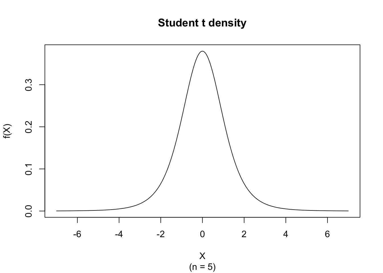
The random variate \(X\) defined for the range \(-\infty \leq X \leq +\infty\), is said to have a Student t-Distribution (i.e. \(X \sim \text{t} \left( n \right)\)) with shape parameter \(n \in \mathbb{N}^+\).

25.1 Probability Density Function

\[ f(X) = \frac{\Gamma \left[ \frac{n+1}{2} \right]}{\Gamma \left[\frac{1}{2}\right] \Gamma \left[ \frac{n}{2} \right] } n ^{-\frac{1}{2}} \left[ 1 + \frac{X^2}{n} \right]^{-\frac{n+1}{2}} \]

The figure below shows an example of the Student t Probability Density function with \(n = 5\).

x <- seq(-7,7,length=1000)
hx <- dt(x, df = 5)
plot(x, hx, type="l", xlab="X", ylab="f(X)", xlim=c(-7,7), main="Student t density", sub = "(n = 5)")

Figure 25.1: Example of Student t Probability Density Function (n = 5)

25.2 Centered Moments

\[ \begin{align*} \mu_j &= 0 & \text{ j odd}\\ \mu_j &= n^{\frac{j}{2}} \frac{\text{B}\left[ \frac{j+1}{2}, \frac{n-j}{2} \right]}{\text{B}\left[ \frac{1}{2}, \frac{n}{2} \right]} & \text{ j even and } j < n \\ \mu_4 &= n^2 \frac{3}{(n-2)(n-4)} & n > 4 \end{align*} \]

25.3 Expected Value

\[ \text{E}(X) = 0 \]

for \(n > 1\).

25.4 Variance

\[ \text{V}(X) = \frac{n}{n-2} \]

for \(n > 2\) (undefined otherwise).

25.5 Median

\[ \text{Med}(X) = 0 \]

25.6 Mode

\[ \text{Mo}(X) = 0 \]

25.7 Skewness

\[ g_1 = 0 \]

for \(n > 3\) (undefined otherwise).

25.8 Kurtosis

\[ g_2 = \frac{3n - 6}{n-4} \]

for \(n > 4\). Note that since \(\lim\limits_{n \rightarrow +\infty} g_2(n) = 3\), it follows that the Kurtosis of the t-Distribution is larger than the Kurtosis of the Normal Distribution.

25.9 Random Number Generator

There is a relationship between the t-Distribution with parameter \(n\) (degrees of freedom), denoted by t\((n)\), the unit normal variate N(0,1), and the Chi-squared Distribution with parameter \(n\), denoted by \(\chi^2(n)\):

\[ X = \frac{\text{N}(0,1)}{\sqrt{\frac{\chi^2(n)}{n}}} \sim \text{t}(n) \]

25.10 Property: Normal Approximation for Large Degrees of Freedom

For \(n \geq 30\) the t-Distribution, denoted by t\((n)\), approximates the Standard Normal Distribution.

25.11 Related Distributions 1: Squared t as a Ratio of Chi-squared Variables

The Student t-Distribution with \(n\) degrees of freedom, represented by t\((n)\), is related to the Chi-squared Distribution:

\[ X^2 = \frac{\chi^2(1)}{\frac{\chi^2(n)}{n}} \text{ where } X \sim \text{t}(n) \]

25.12 Related Distributions 2: Standard Normal / Chi-squared Representation (Squared Form)

The Student t-Distribution with \(n\) degrees of freedom, denoted by t\((n)\), is related to the Standard Normal and the Chi-squared Distribution:

\[ X^2 = \frac{\left[ \text{N}(0,1) \right]^2}{\frac{\chi^2(n)}{n}} \text{ where } X \sim \text{t}(n) \]

25.13 Related Distributions 3: Standard Normal / Chi-squared Representation (Level Form)

The Student t-Distribution with \(n\) degrees of freedom, represented by t\((n)\), is related to the Standard Normal and the Chi-squared Distribution:

\[ X = \frac{\left[ \text{N}(0,1) \right]}{\sqrt{\frac{\chi^2(n)}{n}}} \sim \text{t}(n) \]

25.14 Related Distributions 4: Link with the F Distribution

The Student t-Distribution with \(n\) degrees of freedom, represented by t\((n)\), is related to the F-Distribution:

\[ X^2 = \text{F}(1,n) \text{ where } X \sim \text{t}(n) \]

As a consequence, the statistical F-test with 1 and \(n\) degrees of freedom, is equivalent to the t-test with \(n\) degrees of freedom.

25.15 Related Distributions 5: Cauchy as a Special Case

The t-Distribution with one degree of freedom, denoted by t\((n=1)\), is equal to the two parameter Cauchy Distribution, denoted Cau2(0,1).

25.16 Related Distributions 6: One-sample t Statistic

Consider \(n\) normal variates N\(_i \left(\mu, \sigma^2 \right)\) for \(i = 1, 2, …, n\) and define \(\bar{x}\) and \(s^2\) as

\[ \begin{cases} \bar{x} = \frac{1}{n} \sum_{i=1}^{n} \text{N}_i \left( \mu, \sigma^2 \right) \\ s^2 = \frac{1}{n} \sum_{i=1}^{n} \left[ \text{N}_i \left( \mu, \sigma^2 \right) - \bar{x} \right]^2 \end{cases} \]

and let

\[ \tau = \frac{\bar{x} - \mu}{\sqrt{\frac{s^2}{n-1}}} \]

then it can be shown that \(\tau \sim t(n-1)\). This is the basic form of the so-called one sample t-test.

25.17 Related Distributions 7: Two-sample Pooled-Variance t Statistic

Consider \(n_1\) normal variates N\(_{1i}\left( \mu_1, \sigma^2 \right)\) for \(i = 1, 2, …, n_1\) and \(n_2\) normal variates N\(_{2j}\left( \mu_2, \sigma^2 \right)\) for \(j = 1, 2, …, n_2\). In addition, let the variates \(\bar{x}_k\) and \(s_k^2\) for \(k = 1, 2\) be defined as

\[ \begin{cases} \bar{x}_k = \frac{1}{n_k} \sum_{l=1}^{n_k} \text{N}_{kl} \left( \mu_k, \sigma^2 \right) \\ s_k^2 = \frac{1}{n_k} \sum_{l=1}^{n_k} \left[ \text{N}_{kl} \left( \mu_k, \sigma^2 \right) - \bar{x}_k \right]^2 \end{cases} \]

and let

\[ \tau = \frac{\left( \bar{x}_1 - \bar{x}_2 \right) - \left( \mu_1 - \mu_2 \right) }{\sqrt{\frac{n_1 s_1^2 + n_2 s_2^2}{n_1 + n_2 - 2}} \sqrt{\frac{1}{n_1} + \frac{1}{n_2} } } \]

then it can be shown that \(\tau \sim t(n_1 + n_2 - 2)\). This is the basic form of the so-called independent two sample t-test.

25.18 Related Distributions 8: Noncentral t Distribution

The noncentral \(t\) distribution generalises the Student \(t\) by adding a noncentrality parameter \(\delta \neq 0\). It arises when testing a Normal mean under the alternative hypothesis and is the primary tool for power analysis and sample-size planning for \(t\)-tests (see Chapter 47).

25.19 Example

Suppose we need the critical value for a two-sided 95% confidence interval with 12 degrees of freedom. We compute:

qt(0.975, df = 12)

[1] 2.178813

If we also want the tail probability for an observed test statistic \(t = 2.1\) (with 12 degrees of freedom), we can compute:

2 * (1 - pt(abs(2.1), df = 12))

[1] 0.05754494

25.20 Purpose

The Student t-Distribution is used for inference on means when the population variance is unknown and must be estimated from the sample. It is central to one-sample, paired-sample, and independent two-sample t-tests, and to confidence intervals for means in small to moderate samples.