56 Quantiles

This section defines quantiles and how they are computed. The q-th h-quantile of a random variable \(x\) is the smallest value \(v\) for which \(P(x \leq v) \geq \frac{q}{h}\), where \(h\) represents the number of bins used to partition the data (for example: tertiles with \(h=3\), quartiles with \(h=4\), deciles with \(h=10\), percentiles with \(h=100\), and permilles with \(h=1000\)).

56.1 Practical Choice Guide

Definition family	Typical use
Weighted average at \(X_{nq}\) or \(X_{(n+1)q}\)	Smooth interpolation for continuous data
Empirical distribution / closest observation	Discrete data where observed values should be preserved
Harrell-Davis (Harrell and Davis 1982)	Small to moderate samples when robust, efficient quantile estimation is preferred
Legacy Excel rule	Backward compatibility with older spreadsheets

56.2 Quantiles based on Weighted Averages at \(X_{nq}\)

56.2.1 Definition

When the observations are ordered in ascending order, the quantile at q is defined as:

\[ Quantile(q) = (1 - f)x_i + f x_{i+1} \]

Note that \(nq = i + f\) where i is the integer part of nq and f is the fractional part.

56.2.2 Example

Assume the following original dataset: 21, 24, 50, 10, 23, 27. The number of observations \(n = 6\). Question: what is the percentile value for q = 0.75?

First we obtain the ordered dataset: 10, 21, 23, 24, 27, 50. Next, we compute \(nq = 6 * 0.75 = 4.5\) and obtain the integer part (= 4) and the fractional part (= 0.5). Now we are able to apply the formula: \(Percentile(0.75) = (1-0.5)x_4 + 0.5x_5 = 0.5*24 + 0.5*27 = 25.5\). This is the 75th-percentile estimate under this definition.

56.3 Quantiles based on Weighted Averages at \(X_{(n+1)q}\)

56.3.1 Definition

When the observations are ordered in ascending order, the quantile at q is defined as:

\[ Quantile(q) = (1 - f)x_i + f x_{i+1} \]

Note that \((n+1)q = i + f\) where i is the integer part of (n+1)q and f is the fractional part.

56.3.2 Example

Assume the following original dataset: 21, 24, 50, 10, 23, 27. The number of observations \(n = 6\). Question: what is the percentile value for q = 0.75?

First we obtain the ordered dataset: 10, 21, 23, 24, 27, 50. Next, we compute \((n+1)q = (6+1) * 0.75 = 5.25\) and obtain the integer part (= 5) and the fractional part (= 0.25). Now we are able to apply the formula: \(Percentile(0.75) = (1-0.25)x_5 + 0.25x_6 = 0.75*27 + 0.25*50 = 32.75\). This is the 75th-percentile estimate under this definition.

56.4 Quantiles based on the Empirical Distribution Function

56.4.1 Definition

When the observations are ordered in ascending order, the quantile at q is defined as:

\[ f=0 \Rightarrow Quantile(q) = x_i \]

\[ f>0 \Rightarrow Quantile(q) = x_{i+1} \]

Note that \(nq = i + f\) where i is the integer part of nq and f is the fractional part.

56.4.2 Example

Assume the following original dataset: 21, 24, 50, 10, 23, 27. The number of observations \(n = 6\). Question: what is the percentile value for q = 0.75?

First we obtain the ordered dataset: 10, 21, 23, 24, 27, 50. Next, we compute \(nq = 6 * 0.75 = 4.5\) and obtain the integer part (= 4) and the fractional part (= 0.5). Now we are able to apply the formula (for \(f > 0\)): \(Percentile(0.75) = x_5 = 27\). This is the 75th-percentile estimate under this definition.

56.5 Quantiles based on Averaging

56.5.1 Definition

When the observations are ordered in ascending order, the quantile at q is defined as:

\[ f=0 \Rightarrow Quantile(q) = \frac{1}{2} \left( x_i + x_{i+1} \right) \]

\[ f>0 \Rightarrow Quantile(q) = x_{i+1} \]

Note that \(nq = i + f\) where i is the integer part of nq and f is the fractional part.

56.5.2 Example

Assume the following original dataset: 21, 24, 50, 10, 23, 27. The number of observations \(n = 6\). Question: what is the percentile value for q = 0.75?

First we obtain the ordered dataset: 10, 21, 23, 24, 27, 50. Next, we compute \(nq = 6 * 0.75 = 4.5\) and obtain the integer part (= 4) and the fractional part (= 0.5). Now we are able to apply the formula (for \(f > 0\)): \(Percentile(0.75) = x_5 = 27\). This is the 75th-percentile estimate under this definition.

56.6 Quantiles based on Interpolation

56.6.1 Definition

When the observations are ordered in ascending order, the quantile at q is defined as:

\[ f=0 \Rightarrow Quantile(q) = x_{i+1} \]

\[ f>0 \Rightarrow Quantile(q) = x_{i+1} + f \left( x_{i+2} - x_{i+1} \right) \]

Note that \((n-1)q = i + f\) where i is the integer part of (n-1)q and f is the fractional part.

56.6.2 Example

Assume the following original dataset: 21, 24, 50, 10, 23, 27. The number of observations \(n = 6\). Question: what is the percentile value for q = 0.75?

First we obtain the ordered dataset: 10, 21, 23, 24, 27, 50. Next, we compute \((n-1)q = (6 - 1) * 0.75 = 3.75\) and obtain the integer part (= 3) and the fractional part (= 0.75). Now we are able to apply the formula (for \(f > 0\)): \(Percentile(0.75) = x_4 + 0.75 (x_5 - x_4) = 24 + 0.75(27 - 24) = 24 + 2.25 = 26.25\). This is the 75th-percentile estimate under this definition.

56.7 Quantiles based on Closest Observation

56.7.1 Definition

When the observations are ordered in ascending order, the quantile at q is defined as:

\[ Quantile(q) = x_i \]

Note that \(nq + \frac{1}{2} = i + f\) where i is the integer part of \(nq + \frac{1}{2}\) and f is the fractional part.

56.7.2 Example

Assume the following original dataset: 21, 24, 50, 10, 23, 27. The number of observations \(n = 6\). Question: what is the percentile value for q = 0.75?

First we obtain the ordered dataset: 10, 21, 23, 24, 27, 50. Next, we compute \(nq + \frac{1}{2} = 6 * 0.75 + 0.5 = 5.0\) and obtain the integer part (= 5) and the fractional part (= 0). Now we are able to apply the formula: \(Percentile(0.75) = x_5 = 27\). This is the 75th-percentile estimate under this definition.

56.8 Quantiles based on Statistics Graphics Toolkit (True Basic)

56.8.1 Definition

When the observations are ordered in ascending order, the quantile at q is defined as:

\[ f=0 \Rightarrow Quantile(q) = x_i \]

\[ f>0 \Rightarrow Quantile(q) = (1-f) x_i + f x_{i+1} \]

Note that \((n+1)q = i + f\) where i is the integer part of (n+1)q and f is the fractional part.

This definition is algebraically identical to the previous “Weighted Averages at \(X_{(n+1)q}\)” definition; it is included here as a historical alias used by the Statistics Graphics Toolkit (True Basic).

56.8.2 Example

Assume the following original dataset: 21, 24, 50, 10, 23, 27. The number of observations \(n = 6\). Question: what is the percentile value for q = 0.75?

First we obtain the ordered dataset: 10, 21, 23, 24, 27, 50. Next, we compute \((n+1)q = (6 + 1) * 0.75 = 5.25\) and obtain the integer part (= 5) and the fractional part (= 0.25). Now we are able to apply the formula (for \(f > 0\)): \(Percentile(0.75) = 0.75 * x_5 + 0.25 * x_6 = 0.75 * 27 + 0.25 * 50 = 20.25 + 12.5 = 32.75\). This is the 75th-percentile estimate under this definition.

56.9 Quantiles based on Excel (old versions)

56.9.1 Definition

When the observations are ordered in ascending order, the quantile at q is defined as:

\[ f=0 \Rightarrow Quantile(q) = x_i \]

\[ f=0.5 \Rightarrow Quantile(q) = \frac{1}{2} \left( x_i + x_{i+1} \right) \]

\[ f<0.5 \Rightarrow Quantile(q) = x_i \]

\[ f>0.5 \Rightarrow Quantile(q) = x_{i+1} \]

Note that \((n+1)q = i + f\) where i is the integer part of (n+1)q and f is the fractional part.

56.9.2 Example

Assume the following original dataset: 21, 24, 50, 10, 23, 27. The number of observations \(n = 6\). Question: what is the percentile value for q = 0.75?

First we obtain the ordered dataset: 10, 21, 23, 24, 27, 50. Next, we compute \((n+1)q = (6 + 1) * 0.75 = 5.25\) and obtain the integer part (= 5) and the fractional part (= 0.25). Now we are able to apply the formula (for \(f < 0.5\)): \(Percentile(0.75) = x_5 = 27\). This is the 75th-percentile estimate under this definition.

56.10 Harrell-Davis Quantiles

56.10.1 Definition

The definition of the Harrell-Davis Quantiles is beyond the scope of this book. It is sufficient to know that the Harrell-Davis approach to estimate Quantiles is much more efficient than other techniques, especially when the sample size is relatively small.

56.11 R Module

56.11.1 Public website

The Harrell-Davis Quantiles can be found on the public website:

https://compute.wessa.net/rwasp_harrell_davis.wasp

The public website also features a Percentiles module which uses other types of (more traditional) Quantiles:

https://compute.wessa.net/rwasp_percentiles.wasp

56.11.2 RFC

The Percentiles and Harrell-Davis Quantiles estimator are available in RFC under the menu “Descriptive / Quantiles”.

If you prefer to compute the traditional Quantiles on your local computer, the following code snippet can be used in the R console:

x <- rnorm(200, 4, 10)
x <-sort(x)
i <- 0; f <- 0
q1 <- function(data,n,p,i,f) {
  np <- n*p;
  i <- floor(np)
  f <- np - i
  qvalue <- (1-f)*data[i] + f*data[i+1]
}
q2 <- function(data,n,p,i,f) {
  np <- (n+1)*p
  i <- floor(np)
  f <- np - i
  qvalue <- (1-f)*data[i] + f*data[i+1]
}
q3 <- function(data,n,p,i,f) {
  np <- n*p
  i <- floor(np)
  f <- np - i
  if (f==0) {
    qvalue <- data[i]
  } else {
    qvalue <- data[i+1]
  }
}
q4 <- function(data,n,p,i,f) {
  np <- n*p
  i <- floor(np)
  f <- np - i
  if (f==0) {
    qvalue <- (data[i]+data[i+1])/2
  } else {
    qvalue <- data[i+1]
  }
}
q5 <- function(data,n,p,i,f) {
  np <- (n-1)*p
  i <- floor(np)
  f <- np - i
  if (f==0) {
    qvalue <- data[i+1]
  } else {
    qvalue <- data[i+1] + f*(data[i+2]-data[i+1])
  }
}
q6 <- function(data,n,p,i,f) {
  np <- n*p+0.5
  i <- floor(np)
  f <- np - i
  qvalue <- data[i]
}
q7 <- function(data,n,p,i,f) {
  # Definition 7 is algebraically identical to q2 in this implementation.
  q2(data,n,p,i,f)
}
q8 <- function(data,n,p,i,f) {
  np <- (n+1)*p
  i <- floor(np)
  f <- np - i
  if (f==0) {
    qvalue <- data[i]
  } else {
    if (f == 0.5) {
      qvalue <- (data[i]+data[i+1])/2
    } else {
      if (f < 0.5) {
        qvalue <- data[i]
      } else {
        qvalue <- data[i+1]
      }
    }
  }
}
lx <- length(x)
qval <- array(NA,dim=c(99,8))
mystep <- 25
mystart <- 25
if (lx>10){
  mystep=10
  mystart=10
}
if (lx>20){
  mystep=5
  mystart=5
}
if (lx>50){
  mystep=2
  mystart=2
}
if (lx>=100){
  mystep=1
  mystart=1
}
for (perc in seq(mystart,99,mystep)) {
  qval[perc,1] <- q1(x,lx,perc/100,i,f)
  qval[perc,2] <- q2(x,lx,perc/100,i,f)
  qval[perc,3] <- q3(x,lx,perc/100,i,f)
  qval[perc,4] <- q4(x,lx,perc/100,i,f)
  qval[perc,5] <- q5(x,lx,perc/100,i,f)
  qval[perc,6] <- q6(x,lx,perc/100,i,f)
  qval[perc,7] <- q7(x,lx,perc/100,i,f)
  qval[perc,8] <- q8(x,lx,perc/100,i,f)
}

mydf = data.frame(`WA Xnp` = qval[,1], 
                  `WA X(n+1)p` = qval[,2],
                  `EDF` = qval[,3],
                  `EDF Av` = qval[,4],
                  `EDF Int` = qval[,5],
                  `Cl Obs` = qval[,6],
                  `TBasic` = qval[,7],
                  `Excel` = qval[,8]
                  )
rownames(mydf) = seq(mystart,99,mystep) / 100
mydf

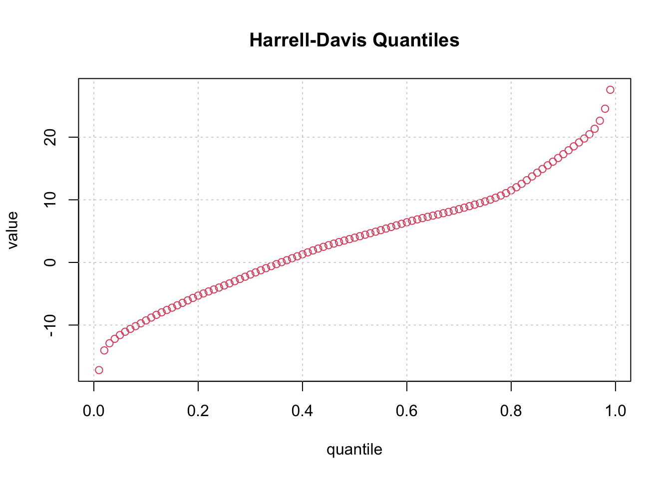
# we only plot the values for the fifth definition
plot(rownames(mydf), mydf[,5], xlab = "quantile", ylab = "value", main = "Quantiles (definition 5)")

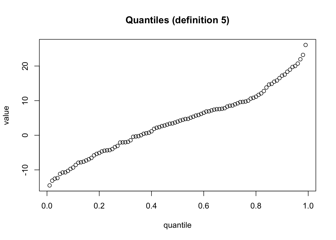
            WA.Xnp   WA.X.n.1.p           EDF       EDF.Av      EDF.Int        Cl.Obs       TBasic         Excel
0.01 -17.792374372 -17.77584433 -17.792374372 -16.96587214 -16.15589996 -17.792374372 -17.77584433 -17.792374372
0.02 -15.182203761 -15.15501598 -15.182203761 -14.50250917 -13.85000237 -15.182203761 -15.15501598 -15.182203761
0.03 -12.601611343 -12.57652157 -12.601611343 -12.18344854 -11.79037551 -12.601611343 -12.57652157 -12.601611343
0.04 -11.599727986 -11.57579356 -11.599727986 -11.30054767 -11.02530178 -11.599727986 -11.57579356 -11.599727986
0.05 -10.016577186 -10.01610246 -10.016577186 -10.01182996 -10.00755745 -10.016577186 -10.01610246 -10.016577186
0.06  -9.807193494  -9.78523899  -9.807193494  -9.62423931  -9.46323962  -9.807193494  -9.78523899  -9.807193494
0.07  -9.001205357  -8.99506437  -8.913476920  -8.91347692  -8.91961791  -9.001205357  -8.99506437  -9.001205357
0.08  -8.825002551  -8.82494375  -8.825002551  -8.82463502  -8.82432629  -8.825002551  -8.82494375  -8.825002551
0.09  -8.623161182  -8.59297099  -8.623161182  -8.45543792  -8.31790484  -8.623161182  -8.59297099  -8.623161182
0.1   -8.220608651  -8.20647367  -8.220608651  -8.14993375  -8.09339382  -8.220608651  -8.20647367  -8.220608651
0.11  -7.988045167  -7.96016163  -7.988045167  -7.86130184  -7.76244204  -7.988045167  -7.96016163  -7.988045167
0.12  -6.888534877  -6.87965883  -6.888534877  -6.85155133  -6.82344384  -6.888534877  -6.87965883  -6.888534877
0.13  -5.653171127  -5.64400826  -5.653171127  -5.61792931  -5.59185037  -5.653171127  -5.64400826  -5.653171127
0.14  -5.521262151  -5.51412236  -5.470263673  -5.47026367  -5.47740346  -5.521262151  -5.51412236  -5.521262151
0.15  -5.311828723  -5.30540967  -5.311828723  -5.29043187  -5.27545407  -5.311828723  -5.30540967  -5.311828723
0.16  -4.884349214  -4.88150311  -4.884349214  -4.87545513  -4.86940716  -4.884349214  -4.88150311  -4.884349214
0.17  -4.826251200  -4.73887094  -4.826251200  -4.56925044  -4.39962994  -4.826251200  -4.73887094  -4.826251200
0.18  -4.263746919  -4.25157577  -4.263746919  -4.22993818  -4.20830059  -4.263746919  -4.25157577  -4.263746919
0.19  -4.193332170  -4.19063704  -4.193332170  -4.18623973  -4.18184242  -4.193332170  -4.19063704  -4.193332170
0.2   -4.135028100  -4.12461559  -4.135028100  -4.10899681  -4.09337804  -4.135028100  -4.12461559  -4.135028100
0.21  -3.792290401  -3.74289977  -3.792290401  -3.67469366  -3.60648756  -3.792290401  -3.74289977  -3.792290401
0.22  -3.394863356  -3.37271059  -3.394863356  -3.34451615  -3.31632172  -3.394863356  -3.37271059  -3.394863356
0.23  -2.928296083  -2.90281219  -2.928296083  -2.87289631  -2.84298044  -2.928296083  -2.90281219  -2.928296083
0.24  -2.754456930  -2.68560507  -2.754456930  -2.61101555  -2.53642603  -2.754456930  -2.68560507  -2.754456930
0.25  -2.396900060  -2.38566069  -2.396900060  -2.37442131  -2.36318194  -2.396900060  -2.38566069  -2.396900060
0.26  -2.329720165  -2.30314097  -2.329720165  -2.27860633  -2.25407169  -2.329720165  -2.30314097  -2.329720165
0.27  -2.093632753  -2.06754754  -2.093632753  -2.04532680  -2.02310607  -2.093632753  -2.06754754  -2.093632753
0.28  -1.890835405  -1.81549836  -1.621774516  -1.62177452  -1.69711157  -1.890835405  -1.81549836  -1.890835405
0.29  -1.605105483  -1.60418619  -1.605105483  -1.60510548  -1.60285479  -1.605105483  -1.60418619  -1.605105483
0.3   -1.538284180  -1.53498952  -1.538284180  -1.53279309  -1.53059665  -1.538284180  -1.53498952  -1.538284180
0.31  -1.305601411  -1.25246814  -1.305601411  -1.21990259  -1.18733704  -1.305601411  -1.25246814  -1.305601411
0.32  -0.966072626  -0.92091935  -0.966072626  -0.89552063  -0.87012192  -0.966072626  -0.92091935  -0.966072626
0.33  -0.473586593  -0.39541290  -0.473586593  -0.35514161  -0.31487031  -0.473586593  -0.39541290  -0.473586593
0.34  -0.200003523  -0.18640388  -0.200003523  -0.18000405  -0.17360422  -0.200003523  -0.18640388  -0.200003523
0.35  -0.002845812   0.05186401  -0.002845812   0.07531107   0.09875814  -0.002845812   0.05186401  -0.002845812
0.36   0.829730174   0.84100803   0.829730174   0.84539386   0.84977969   0.829730174   0.84100803   0.829730174
0.37   0.989951174   1.01521696   0.989951174   1.02409413   1.03297130   0.989951174   1.01521696   0.989951174
0.38   1.069210698   1.08486954   1.069210698   1.08981444   1.09475933   1.069210698   1.08486954   1.069210698
0.39   1.260791192   1.27449482   1.260791192   1.27835994   1.28222507   1.260791192   1.27449482   1.260791192
0.4    1.359143317   1.37157378   1.359143317   1.37468140   1.37778901   1.359143317   1.37157378   1.359143317
0.41   1.541189892   1.59004305   1.541189892   1.60076691   1.61149078   1.541189892   1.59004305   1.541189892
0.42   1.676538464   1.70679765   1.676538464   1.71256131   1.71832496   1.676538464   1.70679765   1.676538464
0.43   1.846019983   1.85626950   1.846019983   1.85793803   1.85960655   1.846019983   1.85626950   1.846019983
0.44   1.881064829   1.94587942   1.881064829   1.95471777   1.96355612   1.881064829   1.94587942   1.881064829
0.45   2.070172164   2.08742062   2.070172164   2.08933712   2.09125361   2.070172164   2.08742062   2.070172164
0.46   2.766010354   2.76720215   2.766010354   2.76730578   2.76740942   2.766010354   2.76720215   2.766010354
0.47   3.073320497   3.12855551   3.073320497   3.13208115   3.13560679   3.073320497   3.12855551   3.073320497
0.48   3.226370866   3.28174805   3.226370866   3.28405543   3.28636281   3.226370866   3.28174805   3.226370866
0.49   3.444650507   3.52192508   3.444650507   3.52350211   3.52507914   3.444650507   3.52192508   3.444650507
0.5    3.611350416   3.65034239   3.611350416   3.65034239   3.65034239   3.611350416   3.65034239   3.650342386
0.51   3.945282336   4.05594925   3.945282336   4.05377931   4.05160937   3.945282336   4.05594925   4.162276288
0.52   4.209065067   4.23922275   4.209065067   4.23806284   4.23690293   4.209065067   4.23922275   4.267060606
0.53   4.294868770   4.31684096   4.294868770   4.31559725   4.31435354   4.294868770   4.31684096   4.336325729
0.54   4.507361417   4.51081411   4.507361417   4.51055835   4.51030260   4.507361417   4.51081411   4.513755290
0.55   4.622368222   4.63658686   4.648220288   4.64822029   4.63400165   4.622368222   4.63658686   4.648220288
0.56   4.698673679   4.74646890   4.784022293   4.78402229   4.73622707   4.698673679   4.74646890   4.784022293
0.57   4.815647739   4.94017456   4.815647739   4.81564774   4.90958902   4.815647739   4.94017456   5.034115846
0.58   5.129249689   5.50221815   5.129249689   5.12924969   5.39933030   5.129249689   5.50221815   5.772298759
0.59   5.916578813   5.92968085   5.916578813   5.92768224   5.92568362   5.916578813   5.92968085   5.938785660
0.6    5.982299236   6.13471160   5.982299236   6.10930954   6.08390748   5.982299236   6.13471160   6.236319850
0.61   6.642975074   6.67419865   6.642975074   6.66856817   6.66293769   6.642975074   6.67419865   6.694161257
0.62   6.823451694   6.84023878   6.823451694   6.83698967   6.83374056   6.823451694   6.84023878   6.850527647
0.63   6.958302192   7.11677817   6.958302192   7.08407678   7.05137539   6.958302192   7.11677817   7.209851365
0.64   7.296714752   7.36750751   7.296714752   7.35202159   7.33653568   7.296714752   7.36750751   7.407328430
0.65   7.728687463   7.74191913   7.728687463   7.73886567   7.73581221   7.728687463   7.74191913   7.749043873
0.66   7.830509674   7.83919416   7.830509674   7.83708883   7.83498350   7.830509674   7.83919416   7.843667982
0.67   7.924933241   7.95002788   7.924933241   7.94366058   7.93729329   7.924933241   7.95002788   7.962387929
0.68   8.105561475   8.12836089   8.105561475   8.12232575   8.11629061   8.105561475   8.12836089   8.139090025
0.69   8.141347572   8.43706395   8.141347572   8.35563480   8.27420565   8.141347572   8.43706395   8.569922028
0.7    8.723651965   8.73282221   8.723651965   8.73020214   8.72758207   8.723651965   8.73282221   8.736752314
0.71   8.743380661   8.92396747   8.743380661   8.87055447   8.81714147   8.743380661   8.92396747   8.997728284
0.72   9.196782469   9.25094288   9.196782469   9.23439386   9.21784485   9.196782469   9.25094288   9.272005259
0.73   9.349249828   9.42544521   9.349249828   9.40143844   9.37743168   9.349249828   9.42544521   9.453627058
0.74   9.738438685   9.80132100   9.738438685   9.78092673   9.76053247   9.738438685   9.80132100   9.823414784
0.75   9.929167617  10.29301895   9.929167617  10.17173517  10.05045139   9.929167617  10.29301895  10.414302724
0.76  10.738993906  10.90290214  10.738993906  10.84682827  10.79075440  10.738993906  10.90290214  10.954662639
0.77  11.219785561  11.58576448  11.219785561  11.45743421  11.32910394  11.219785561  11.58576448  11.695082854
0.78  11.735697146  11.94686217  11.735697146  11.87105934  11.79525651  11.735697146  11.94686217  12.006421529
0.79  12.043410028  12.28053766  12.043410028  12.19349081  12.10644396  12.043410028  12.28053766  12.343571584
0.8   12.840159257  12.96912896  12.840159257  12.92076532  12.87240168  12.840159257  12.96912896  13.001371390
0.81  13.058205272  13.06758155  13.058205272  13.06399310  13.06040465  13.058205272  13.06758155  13.069780920
0.82  13.194584556  13.23079105  13.194584556  13.21666169  13.20253232  13.194584556  13.23079105  13.238738823
0.83  13.267821488  13.65854819  13.267821488  13.50319902  13.34784985  13.267821488  13.65854819  13.738576555
0.84  14.312539068  14.38730078  14.312539068  14.35704009  14.32677939  14.312539068  14.38730078  14.401541102
0.85  14.791028949  15.15353973  14.791028949  15.00427058  14.85500144  14.791028949  15.15353973  15.217512219
0.86  15.688767614  15.96706778  15.688767614  15.85057004  15.73407229  15.688767614  15.96706778  16.012372461
0.87  16.065085422  16.17993949  16.065085422  16.13109351  16.08224752  16.065085422  16.17993949  16.197101595
0.88  16.233150681  16.37309142  16.233150681  16.31266247  16.25223351  16.233150681  16.37309142  16.392174254
0.89  16.705914625  16.73991561  16.705914625  16.72501630  16.71011699  16.705914625  16.73991561  16.744117979
0.9   16.982964171  17.08777606  16.982964171  17.04119300  16.99460994  16.982964171  17.08777606  17.099421829
0.91  17.349053464  17.51637333  17.349053464  17.44098745  17.36560158  17.349053464  17.51637333  17.532921445
0.92  17.535557501  17.82234968  17.535557501  17.69142282  17.56049595  17.535557501  17.82234968  17.847288132
0.93  19.684395840  19.78612034  19.684395840  19.73908643  19.69205252  19.684395840  19.78612034  19.793777022
0.94  19.911966311  20.21089751  19.911966311  20.07097227  19.93104703  19.911966311  20.21089751  20.229978221
0.95  20.495700130  21.42460679  20.495700130  20.98459837  20.54458995  20.495700130  21.42460679  21.473496610
0.96  21.548570872  21.67076902  21.548570872  21.61221574  21.55366246  21.548570872  21.67076902  21.675860605
0.97  22.168280306  22.55060533  22.168280306  22.36535506  22.18010479  22.168280306  22.55060533  22.562429820
0.98  22.771469596  23.25125000  22.771469596  23.01625552  22.78126103  22.771469596  23.25125000  23.261041442
0.99  23.724728628  24.28570993  23.724728628  24.00805252  23.73039511  23.724728628  24.28570993  24.291376411

To compute traditional Quantiles, the R code must sort the data and define new functions for each definition: the functions are called q1, q2, …, q8. To make the script a bit more intelligent, the number of quantiles is made dependent on the number of observations \(N\). For instance, if \(N <= 10\) the script produces deciles and if \(N >= 100\) it computes percentiles.

A better alternative are the Harrell-Davis Quantiles that can also be computed in the R console:

library(Hmisc)

# we use the same data in variable x as before
par1 = 0.01 #lowest quantile
par2 = 0.99 #highest quantile
par3 = 0.01 #step size
ylab = 'value'
xlab = 'quantile'
main = 'Harrell-Davis Quantiles'
myseq <- seq(par1, par2, par3)
hd <- hdquantile(x, probs = myseq, se = TRUE, na.rm = FALSE, names = TRUE, weights=FALSE)
hd
plot(myseq,hd,col=2,main=main,xlab=xlab,ylab=ylab)
grid()

       0.01        0.02        0.03        0.04        0.05        0.06        0.07        0.08        0.09        0.10        0.11 
-16.9990213 -14.6651919 -12.7845394 -11.4256394 -10.4627207  -9.7620741  -9.2305318  -8.7889049  -8.3644765  -7.9039854  -7.3892170 
       0.12        0.13        0.14        0.15        0.16        0.17        0.18        0.19        0.20        0.21        0.22 
 -6.8399803  -6.2983113  -5.8034625  -5.3745477  -5.0091104  -4.6921320  -4.4054804  -4.1331540  -3.8635292  -3.5906311  -3.3144456 
       0.23        0.24        0.25        0.26        0.27        0.28        0.29        0.30        0.31        0.32        0.33 
 -3.0394282  -2.7714169  -2.5143824  -2.2684897  -2.0299861  -1.7924828  -1.5488574  -1.2931567  -1.0221344  -0.7361761  -0.4394173 
       0.34        0.35        0.36        0.37        0.38        0.39        0.40        0.41        0.42        0.43        0.44 
 -0.1389770   0.1565641   0.4390842   0.7027536   0.9453057   1.1684367   1.3772763   1.5791161   1.7817309   1.9916861   2.2129968 
       0.45        0.46        0.47        0.48        0.49        0.50        0.51        0.52        0.53        0.54        0.55 
  2.4464396   2.6896732   2.9381143   3.1862963   3.4293186   3.6640382   3.8898012   4.1086573   4.3250535   4.5450126   4.7748559 
       0.56        0.57        0.58        0.59        0.60        0.61        0.62        0.63        0.64        0.65        0.66 
  5.0196857   5.2820141   5.5609880   5.8525012   6.1501643   6.4467941   6.7359448   7.0130979   7.2763316   7.5264702   7.7667970 
       0.67        0.68        0.69        0.70        0.71        0.72        0.73        0.74        0.75        0.76        0.77 
  8.0024493   8.2396637   8.4850997   8.7454093   9.0270053   9.3357150   9.6759504  10.0493425  10.4533374  10.8806597  11.3204643 
       0.78        0.79        0.80        0.81        0.82        0.83        0.84        0.85        0.86        0.87        0.88 
 11.7613740  12.1956794  12.6230484  13.0515404  13.4941765  13.9614078  14.4530235  14.9550479  15.4453475  15.9062643  16.3378227 
       0.89        0.90        0.91        0.92        0.93        0.94        0.95        0.96        0.97        0.98        0.99 
 16.7648926  17.2341159  17.7969785  18.4800575  19.2612564  20.0797878  20.8758529  21.6245500  22.3505846  23.1504508  24.3846060 
attr(,"se")
     0.01      0.02      0.03      0.04      0.05      0.06      0.07      0.08      0.09      0.10      0.11      0.12      0.13 
1.6405091 1.8696034 1.6563875 1.3361268 1.0810229 0.8793805 0.7527926 0.7364119 0.8364680 1.0045658 1.1565150 1.2197137 1.1735985 
     0.14      0.15      0.16      0.17      0.18      0.19      0.20      0.21      0.22      0.23      0.24      0.25      0.26 
1.0533145 0.9161605 0.8043618 0.7333458 0.7023673 0.7048629 0.7291204 0.7582993 0.7761077 0.7739912 0.7541791 0.7272437 0.7065677 
     0.27      0.28      0.29      0.30      0.31      0.32      0.33      0.34      0.35      0.36      0.37      0.38      0.39 
0.7030742 0.7221804 0.7629845 0.8188606 0.8789947 0.9307513 0.9625562 0.9666663 0.9411404 0.8904841 0.8247473 0.7572502 0.7015107 
     0.40      0.41      0.42      0.43      0.44      0.45      0.46      0.47      0.48      0.49      0.50      0.51      0.52 
0.6681223 0.6622802 0.6826157 0.7217922 0.7686650 0.8112593 0.8397596 0.8487402 0.8380410 0.8122118 0.7790402 0.7478685 0.7280307 
     0.53      0.54      0.55      0.56      0.57      0.58      0.59      0.60      0.61      0.62      0.63      0.64      0.65 
0.7271964 0.7493645 0.7930393 0.8508337 0.9111768 0.9615278 0.9918132 0.9968592 0.9771160 0.9377635 0.8869341 0.8338878 0.7875472 
     0.66      0.67      0.68      0.69      0.70      0.71      0.72      0.73      0.74      0.75      0.76      0.77      0.78 
0.7553119 0.7420548 0.7496740 0.7777388 0.8249094 0.8897334 0.9696659 1.0587790 1.1462028 1.2173348 1.2581702 1.2611247 1.2297973 
     0.79      0.80      0.81      0.82      0.83      0.84      0.85      0.86      0.87      0.88      0.89      0.90      0.91 
1.1803946 1.1381050 1.1270802 1.1554240 1.2047151 1.2365173 1.2149495 1.1306374 1.0104712 0.9077622 0.8806063 0.9650608 1.1407964 
     0.92      0.93      0.94      0.95      0.96      0.97      0.98      0.99 
1.3157014 1.3793385 1.2971792 1.1247043 0.9367010 0.7949161 0.7372297 0.9319469

To compute Harrell-Davis Quantiles, the R code uses the hdquantile function from the Hmisc library to produce the output. The dataset is simulated with the rnorm function as a series of random numbers (N = 200).

56.12 Purpose

Quantiles are used to describe the distribution of a random variable. They are also used to construct new types of statistical methods such as the QQ Plot, the Normal Probability Plot, PPCC Plot, etc.

56.13 Pros & Cons

56.13.1 Pros

The use of Quantiles has the following advantages:

They are easily computed with most software packages (even though most packages don’t explain which definition is used).
They are relatively easy to interpret and convey a lot of information in a simple graph or table.
Educated readers may be familiar with Quantiles -- therefore it is one of the preferred methods to report information about the distribution of a variable of interest.

56.13.2 Cons

The use of Quantiles has the following disadvantages:

Most software packages don’t explain the exact definition that is used to compute the Quantiles (see Hyndman and Fan 1996 for a systematic comparison of nine definitions). This can have serious consequences, especially for small samples or when computing Quantiles for distributions with heavy tails.
Most software packages do not use the Harrell-Davis Quantiles.
Traditional types of Percentiles, Quartiles, etc. often require the researcher to make interpolations between adjacent quantile points.

56.14 Example

The analysis shown below illustrates the (traditional) Percentiles for a dataset containing student motivation scores. The column headings are abbreviated and correspond to the various definitions of quantiles (the Harrell-Davis Quantiles are not included).

Interactive Shiny app (click to load).

Open in new tab

Suppose we wish to compute an interval which contains the middle 95% of observations. How should we determine this interval?

To find the interval \(\left[ Quantile(0.025), Quantile(0.975) \right]\) we have to lookup the quantiles that are closest to the lower and upper bounds (0.025 and 0.975). The problem is that we can’t find the exact values in the output, implying that we need to approximate the bounds by interpolation:

The lower bound is found by computing the average Quantile of P(0.02) and P(0.03). For instance, if we use definition 6, we compute the average of 11 and 13 (which is 12).
The upper bound is found by computing the average Quantile of P(0.97) and P(0.98). For instance, if we use definition 6, we compute the average of 26 and 27 (which is 26.5).

According to definition 6, the interval [12, 26.5] contains the middle 95% of all observations.

56.15 Task

For the same data as in previous example, compute the 95% interval by using:

the traditional quantiles with an appropriate stepsize
the Harrell-Davis method

Which method is best?