The Cauchy distribution is the canonical example of a distribution with no finite moments — not even the mean. Its power-law tails decay so slowly that the average of \(n\) Cauchy random variables has the same distribution as a single one, and the Central Limit Theorem fails entirely.
Formally, the random variate \(X\) defined for all of \(\mathbb{R}\), is said to have a Cauchy Distribution (i.e. \(X \sim \text{Cauchy}(x_0, \gamma)\)) with location parameter \(x_0 \in \mathbb{R}\) and scale parameter \(\gamma > 0\). The standard Cauchy has \(x_0 = 0\) and \(\gamma = 1\). In R: dcauchy(x, location = x0, scale = gamma), pcauchy, qcauchy, rcauchy.
Note: Two app modules cover this distribution — a standard Cauchy app (no parameter sliders, fixed at \(x_0 = 0\), \(\gamma = 1\)) and a location-scale app. Both are described in the R Module section.
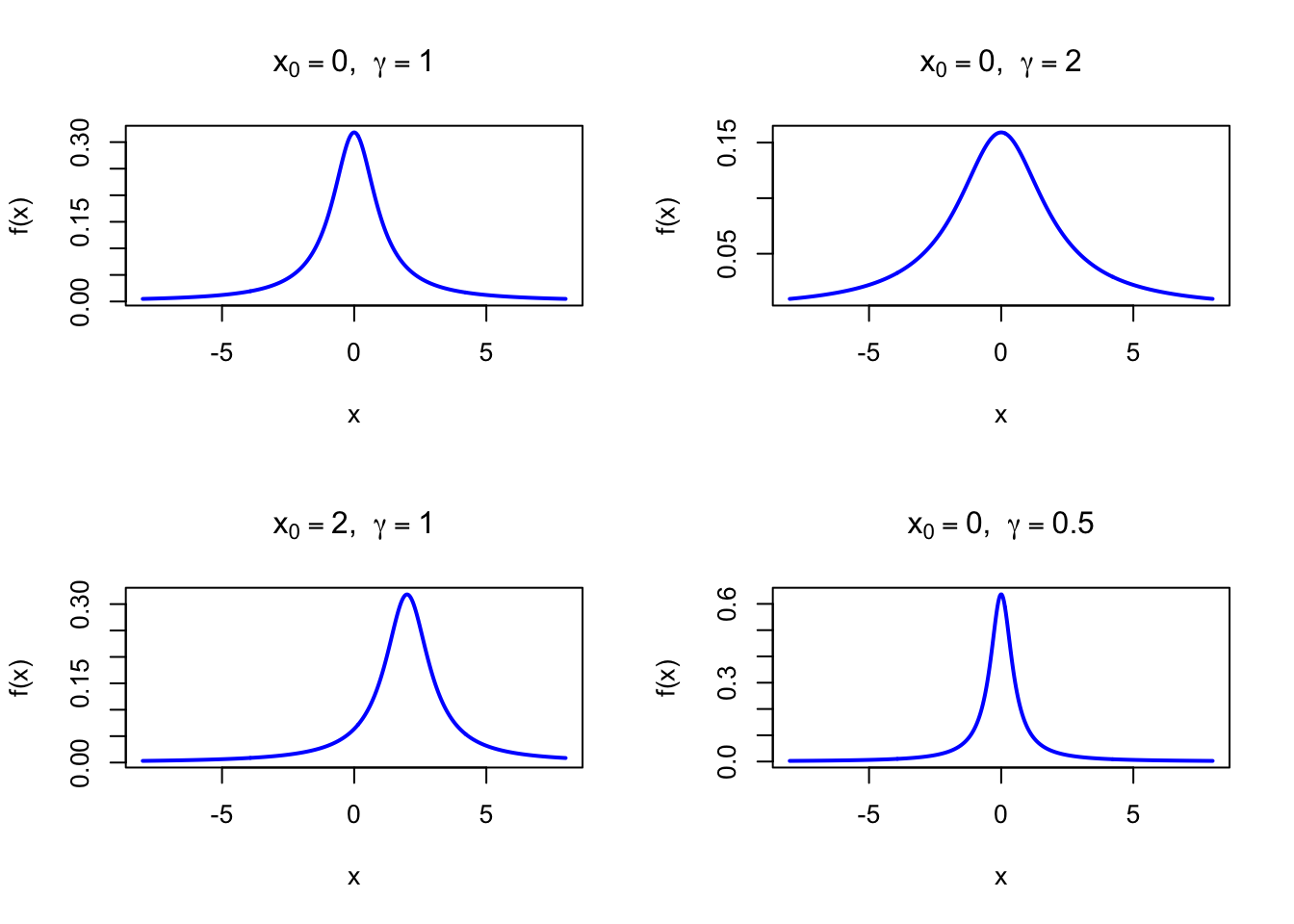
The figure below shows examples of the Cauchy Probability Density Function for different parameter combinations.
Code
par(mfrow =c(2, 2))x <-seq(-8, 8, length =500)plot(x, dcauchy(x, location =0, scale =1), type ="l", lwd =2, col ="blue",xlab ="x", ylab ="f(x)", main =expression(paste(x[0] ==0, ", ", gamma ==1)))plot(x, dcauchy(x, location =0, scale =2), type ="l", lwd =2, col ="blue",xlab ="x", ylab ="f(x)", main =expression(paste(x[0] ==0, ", ", gamma ==2)))plot(x, dcauchy(x, location =2, scale =1), type ="l", lwd =2, col ="blue",xlab ="x", ylab ="f(x)", main =expression(paste(x[0] ==2, ", ", gamma ==1)))plot(x, dcauchy(x, location =0, scale =0.5), type ="l", lwd =2, col ="blue",xlab ="x", ylab ="f(x)", main =expression(paste(x[0] ==0, ", ", gamma ==0.5)))par(mfrow =c(1, 1))
Figure 39.1: Cauchy Probability Density Function for various parameter combinations
39.2 Purpose
The Cauchy distribution is a fundamental counterexample in probability theory: it violates the conditions of the Law of Large Numbers and the Central Limit Theorem. Despite its pathological moment structure, it arises naturally as the ratio of two independent standard Normal random variables. Common appearances include:
Ratio of two independent Normal random variables
Resonance curves in physics (Lorentz/Breit-Wigner distribution)
Cauchy principal value integrals in complex analysis
Stable distribution theory: the Cauchy is a stable distribution with index \(\alpha = 1\)
Demonstrates the necessity of finite variance for the CLT to apply
Relation to the discrete setting. No standard discrete distribution has completely undefined moments. The closest conceptual relative is the Zeta distribution with shape parameter \(\leq 1\), for which the mean is also infinite. The Cauchy illustrates an extreme case where standard statistical summaries break down completely.
The following code demonstrates Cauchy probability calculations and the CLT failure:
x0 <-0; gamma_par <-1# Density at x = 0dcauchy(0, location = x0, scale = gamma_par)# P(|X| < 1): probability within one "scale unit" of centerpcauchy(1, location = x0, scale = gamma_par) -pcauchy(-1, location = x0, scale = gamma_par)# Mediancat("Median:", qcauchy(0.5, location = x0, scale = gamma_par), "\n")
[1] 0.3183099
[1] 0.5
Median: 0
39.20 Example
The Cauchy distribution demonstrates the failure of the Central Limit Theorem. The sample mean of \(n\) i.i.d. Cauchy\((0, 1)\) variates is itself Cauchy\((0, 1)\) — averaging provides no concentration of the estimate.
set.seed(42)n <-1000# Sample means of n Cauchy draws — should converge to 0 if CLT heldmeans_200 <-replicate(200, mean(rcauchy(n)))cat("Mean of sample means:", round(mean(means_200), 4), "\n")cat("SD of sample means: ", round(sd(means_200), 4), "\n")cat("Expected SD if CLT: ", round(1/sqrt(n), 6), "(CLT would predict ~0.032)\n")cat("Note: sd >> 1/sqrt(n), confirming CLT does NOT apply\n")
Mean of sample means: -2.952
SD of sample means:   39.4931
Expected SD if CLT:   0.031623 (CLT would predict ~0.032)
Note: sd >> 1/sqrt(n), confirming CLT does NOT apply
The standard Cauchy app illustrates the distribution shape without adjustable parameters:
If \(Z_1, Z_2 \overset{\text{i.i.d.}}{\sim} N(0, 1)\) then:
\[
\frac{Z_1}{Z_2} \sim \text{Cauchy}(0, 1)
\]
This is the most natural way the Cauchy distribution arises in practice.
39.23 Property 2: Stable Distribution — Averaging Does Not Help
The Cauchy distribution is a stable distribution with index \(\alpha = 1\). If \(X_1, \ldots, X_n \overset{\text{i.i.d.}}{\sim} \text{Cauchy}(x_0, \gamma)\) then:
Averaging \(n\) Cauchy variates produces no concentration whatsoever — the distribution of the mean is identical to the distribution of a single observation.
39.24 Property 3: Student’s t with 1 Degree of Freedom
The standard Cauchy distribution is identical to Student’s t-distribution with 1 degree of freedom: