• Descriptive
    • Moments
    • Concentration
    • Central Tendency
    • Variability
    • Stem-and-Leaf Plot
    • Histogram & Frequency Table
    • Data Quality Forensics
    • Conditional EDA
    • Quantiles
    • Kernel Density Estimation
    • Normal QQ Plot
    • Bootstrap Plot

    • Multivariate Descriptive Statistics
  • Distributions
    • Binomial Probabilities
    • Geometric Probabilities
    • Negative Binomial Probabilities
    • Hypergeometric Probabilities
    • Multinomial Probabilities
    • Dirichlet
    • Poisson Probabilities

    • Exponential
    • Gamma
    • Erlang
    • Weibull
    • Rayleigh
    • Maxwell-Boltzmann
    • Lognormal
    • Pareto
    • Inverse Gamma
    • Inverse Chi-Square

    • Beta
    • Power
    • Beta Prime (Inv. Beta)
    • Triangular

    • Normal (area)
    • Logistic
    • Laplace
    • Cauchy (standard)
    • Cauchy (location-scale)
    • Gumbel
    • Fréchet
    • Generalized Extreme Value

    • Normal RNG
    • ML Fitting
    • Tukey Lambda PPCC
    • Box-Cox Normality Plot
    • Noncentral t
    • Noncentral F
    • Sample Correlation r

    • Empirical Tests
  • Hypotheses
    • Theoretical Aspects of Hypothesis Testing
    • Bayesian Inference
    • Minimum Sample Size

    • Empirical Tests
    • Multivariate (pair-wise) Testing
  • Models
    • Manual Model Building
    • Guided Model Building
  • Time Series
    • Time Series Plot
    • Decomposition
    • Exponential Smoothing

    • Blocked Bootstrap Plot
    • Mean Plot
    • (P)ACF
    • VRM
    • Standard Deviation-Mean Plot
    • Spectral Analysis
    • ARIMA

    • Cross Correlation Function
    • Granger Causality
  1. Probability Distributions
  2. 19  Uniform Distribution (Rectangular Distribution)
  • Preface
  • Getting Started
    • 1  Introduction
    • 2  Why Do We Need Innovative Technology?
    • 3  Basic Definitions
    • 4  The Big Picture: Why We Analyze Data
  • Introduction to Probability
    • 5  Definitions of Probability
    • 6  Jeffreys’ axiom system
    • 7  Bayes’ Theorem
    • 8  Sensitivity and Specificity
    • 9  Naive Bayes Classifier
    • 10  Law of Large Numbers

    • 11  Problems
  • Probability Distributions
    • 12  Bernoulli Distribution
    • 13  Binomial Distribution
    • 14  Geometric Distribution
    • 15  Negative Binomial Distribution
    • 16  Hypergeometric Distribution
    • 17  Multinomial Distribution
    • 18  Poisson Distribution

    • 19  Uniform Distribution (Rectangular Distribution)
    • 20  Normal Distribution (Gaussian Distribution)
    • 21  Gaussian Naive Bayes Classifier
    • 22  Chi Distribution
    • 23  Chi-squared Distribution (1 parameter)
    • 24  Chi-squared Distribution (2 parameters)
    • 25  Student t-Distribution
    • 26  Fisher F-Distribution
    • 27  Exponential Distribution
    • 28  Lognormal Distribution
    • 29  Gamma Distribution
    • 30  Beta Distribution
    • 31  Weibull Distribution
    • 32  Pareto Distribution
    • 33  Inverse Gamma Distribution
    • 34  Rayleigh Distribution
    • 35  Erlang Distribution
    • 36  Logistic Distribution
    • 37  Laplace Distribution
    • 38  Gumbel Distribution
    • 39  Cauchy Distribution
    • 40  Triangular Distribution
    • 41  Power Distribution
    • 42  Beta Prime Distribution
    • 43  Sample Correlation Distribution
    • 44  Dirichlet Distribution
    • 45  Generalized Extreme Value (GEV) Distribution
    • 46  Frechet Distribution
    • 47  Noncentral t Distribution
    • 48  Noncentral F Distribution
    • 49  Inverse Chi-Squared Distribution
    • 50  Maxwell-Boltzmann Distribution
    • 51  Distribution Relationship Map

    • 52  Problems
  • Descriptive Statistics & Exploratory Data Analysis
    • 53  Types of Data
    • 54  Datasheets

    • 55  Frequency Plot (Bar Plot)
    • 56  Frequency Table
    • 57  Contingency Table
    • 58  Binomial Classification Metrics
    • 59  Confusion Matrix
    • 60  ROC Analysis

    • 61  Stem-and-Leaf Plot
    • 62  Histogram
    • 63  Data Quality Forensics
    • 64  Quantiles
    • 65  Central Tendency
    • 66  Variability
    • 67  Skewness & Kurtosis
    • 68  Concentration
    • 69  Notched Boxplot
    • 70  Scatterplot
    • 71  Pearson Correlation
    • 72  Rank Correlation
    • 73  Partial Pearson Correlation
    • 74  Simple Linear Regression
    • 75  Moments
    • 76  Quantile-Quantile Plot (QQ Plot)
    • 77  Normal Probability Plot
    • 78  Probability Plot Correlation Coefficient Plot (PPCC Plot)
    • 79  Box-Cox Normality Plot
    • 80  Kernel Density Estimation
    • 81  Bivariate Kernel Density Plot
    • 82  Conditional EDA: Panel Diagnostics
    • 83  Bootstrap Plot (Central Tendency)
    • 84  Survey Scores Rank Order Comparison
    • 85  Cronbach Alpha

    • 86  Equi-distant Time Series
    • 87  Time Series Plot (Run Sequence Plot)
    • 88  Mean Plot
    • 89  Blocked Bootstrap Plot (Central Tendency)
    • 90  Standard Deviation-Mean Plot
    • 91  Variance Reduction Matrix
    • 92  (Partial) Autocorrelation Function
    • 93  Periodogram & Cumulative Periodogram

    • 94  Problems
  • Hypothesis Testing
    • 95  Normal Distributions revisited
    • 96  The Population
    • 97  The Sample
    • 98  The One-Sided Hypothesis Test
    • 99  The Two-Sided Hypothesis Test
    • 100  When to use a one-sided or two-sided test?
    • 101  What if \(\sigma\) is unknown?
    • 102  The Central Limit Theorem (revisited)
    • 103  Statistical Test of the Population Mean with known Variance
    • 104  Statistical Test of the Population Mean with unknown Variance
    • 105  Statistical Test of the Variance
    • 106  Statistical Test of the Population Proportion
    • 107  Statistical Test of the Standard Deviation \(\sigma\)
    • 108  Statistical Test of the difference between Means -- Independent/Unpaired Samples
    • 109  Statistical Test of the difference between Means -- Dependent/Paired Samples
    • 110  Statistical Test of the difference between Variances -- Independent/Unpaired Samples

    • 111  Hypothesis Testing for Research Purposes
    • 112  Decision Thresholds, Alpha, and Confidence Levels
    • 113  Bayesian Inference for Decision-Making
    • 114  One Sample t-Test
    • 115  Skewness & Kurtosis Tests
    • 116  Paired Two Sample t-Test
    • 117  Wilcoxon Signed-Rank Test
    • 118  Unpaired Two Sample t-Test
    • 119  Unpaired Two Sample Welch Test
    • 120  Two One-Sided Tests (TOST) for Equivalence
    • 121  Mann-Whitney U test (Wilcoxon Rank-Sum Test)
    • 122  Bayesian Two Sample Test
    • 123  Median Test based on Notched Boxplots
    • 124  Chi-Squared Tests for Count Data
    • 125  Kolmogorov-Smirnov Test
    • 126  One Way Analysis of Variance (1-way ANOVA)
    • 127  Kruskal-Wallis Test
    • 128  Two Way Analysis of Variance (2-way ANOVA)
    • 129  Repeated Measures ANOVA
    • 130  Friedman Test
    • 131  Testing Correlations
    • 132  A Note on Causality

    • 133  Problems
  • Regression Models
    • 134  Simple Linear Regression Model (SLRM)
    • 135  Multiple Linear Regression Model (MLRM)
    • 136  Logistic Regression
    • 137  Generalized Linear Models
    • 138  Multinomial and Ordinal Logistic Regression
    • 139  Cox Proportional Hazards Regression
    • 140  Conditional Inference Trees
    • 141  Leaf Diagnostics for Conditional Inference Trees
    • 142  Conditional Random Forests
    • 143  Hypothesis Testing with Linear Regression Models (from a Practical Point of View)

    • 144  Problems
  • Introduction to Time Series Analysis
    • 145  Case: the Market of Health and Personal Care Products
    • 146  Decomposition of Time Series
    • 147  Ad hoc Forecasting of Time Series
  • Box-Jenkins Analysis
    • 148  Introduction to Box-Jenkins Analysis
    • 149  Theoretical Concepts
    • 150  Stationarity
    • 151  Identifying ARMA parameters
    • 152  Estimating ARMA Parameters and Residual Diagnostics
    • 153  Forecasting with ARIMA models
    • 154  Intervention Analysis
    • 155  Cross-Correlation Function
    • 156  Transfer Function Noise Models
    • 157  General-to-Specific Modeling
  • Model Building Strategies
    • 158  Introduction to Model Building Strategies
    • 159  Manual Model Building
    • 160  Model Validation
    • 161  Regularization Methods
    • 162  Hyperparameter Optimization Strategies
    • 163  Guided Model Building in Practice
    • 164  Diagnostics, Revision, and Guided Forecasting
    • 165  Leakage, Target Encoding, and Robust Regression
  • References
  • Appendices
    • Appendices
    • A  Method Selection Guide
    • B  Presentations and Teaching Materials
    • C  R Language Concepts for Statistical Computing
    • D  Matrix Algebra
    • E  Standard Normal Table (Gaussian Table)
    • F  Critical values of Student’s \(t\) distribution with \(\nu\) degrees of freedom
    • G  Upper-tail critical values of the \(\chi^2\)-distribution with \(\nu\) degrees of freedom
    • H  Lower-tail critical values of the \(\chi^2\)-distribution with \(\nu\) degrees of freedom

Table of contents

  • 19.1 Probability Density Function
  • 19.2 Distribution Function
  • 19.3 Moment Generating Function
  • 19.4 Centered Moments
  • 19.5 Expected Value
  • 19.6 Variance
  • 19.7 Median
  • 19.8 Coefficient of Skewness
  • 19.9 Coefficient of Kurtosis
  • 19.10 Coefficient of Variation
  • 19.11 Purpose
  • 19.12 Example
  1. Probability Distributions
  2. 19  Uniform Distribution (Rectangular Distribution)

19  Uniform Distribution (Rectangular Distribution)

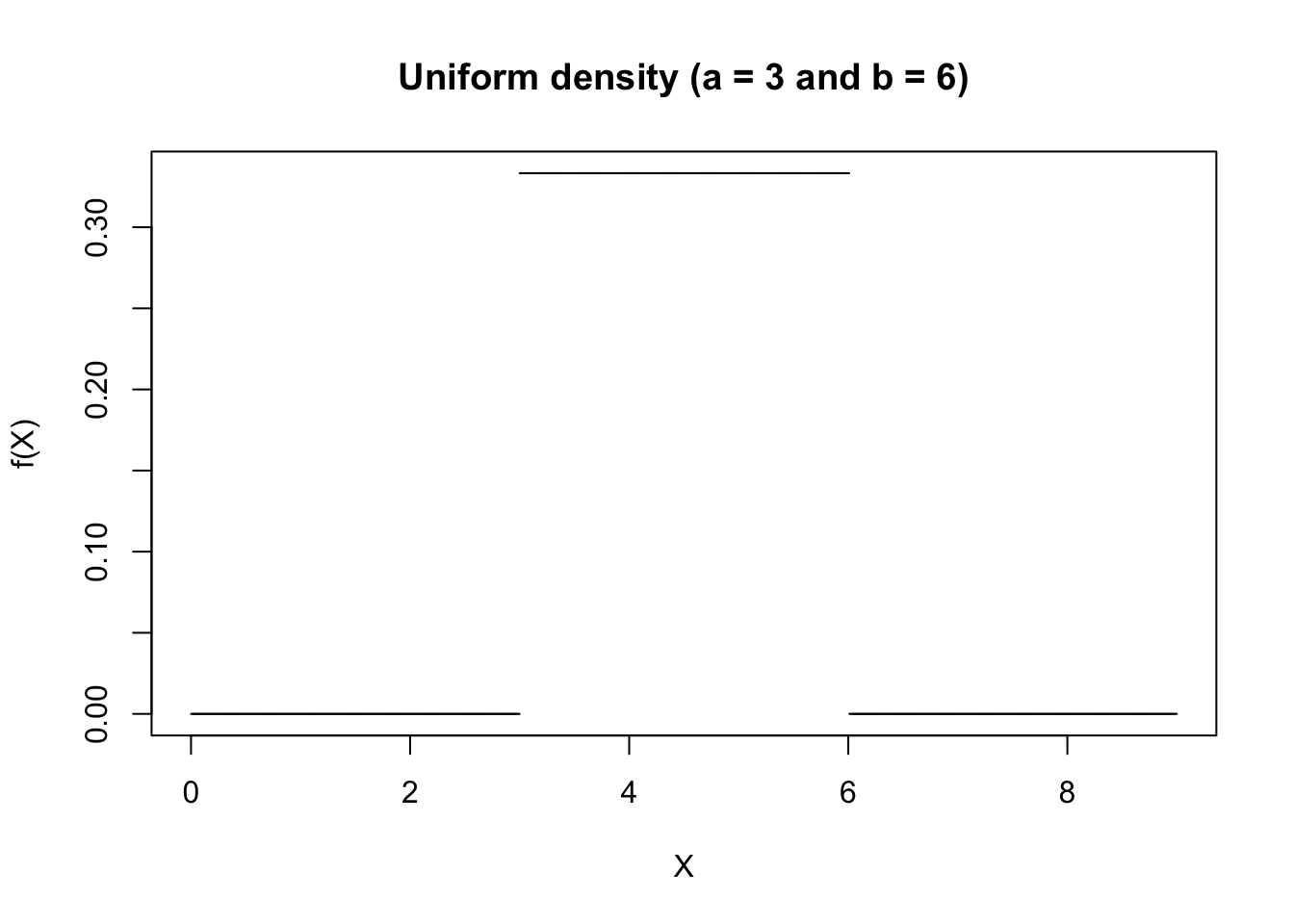
The random variate \(X\) defined for the range \(a \leq X \leq b\), is said to have a Uniform Distribution (i.e. \(X \sim \text{U}\left( a, b \right)\)) with location parameters \(a\) and \(b\) where \(-\infty < a < b < + \infty\)

19.1 Probability Density Function

\[ \begin{align*} \begin{cases} \text{f}(X) = \frac{1}{b-a} \text{ for } X \in [a, b] \\ \text{f}(X) = 0 \text{ for } X \notin [a, b] \end{cases} \end{align*} \]

The figure below shows an example of the Uniform Probability Density function for \(a = 3\) and \(b = 6\).

Code
x <- seq(0,9,length=1000) 
hx <- dunif(x, min = 3, max = 6) 
plot(x,hx,type="n",xlab="X", ylab="f(X)", xlim=c(0,9), main="Uniform density (a = 3 and b = 6)") 
segments(x[-length(x)],hx[-length(x)],x[-1],hx[-length(x)])
Figure 19.1: Example of Uniform Probability Density Function (a = 3 and b = 6)

Since the surface under the density function is (by definition) always equal to 1, it follows that the probability in the density figure below of \(X\) being contained in the interval \([a = 3, b = 6]\) is also equal to 1 (i.e. \(\text{P}(3 < X < 6) = 1\)).

19.2 Distribution Function

\[ \begin{align*} \begin{cases} \text{F}(X) = 0 \text{ for } X < a \\ \text{F}(X) = \frac{X-a}{b-a} \text{ for } X \in [a, b] \\ \text{F}(X) = 1 \text{ for } X > b \end{cases} \end{align*} \]

The figure below shows an example of the Uniform Distribution function for \(a = 3\) and \(b = 6\).

Code
x <- seq(0,9,length=1000)
hx <- punif(x, min = 3, max = 6)
plot(x, hx, type="l", xlab="X", ylab="F(X)", xlim=c(0,9), main="Uniform distribution (a = 3 and b = 6)")
Figure 19.2: Example of Uniform Distribution Function (a = 3 and b = 6)

19.3 Moment Generating Function

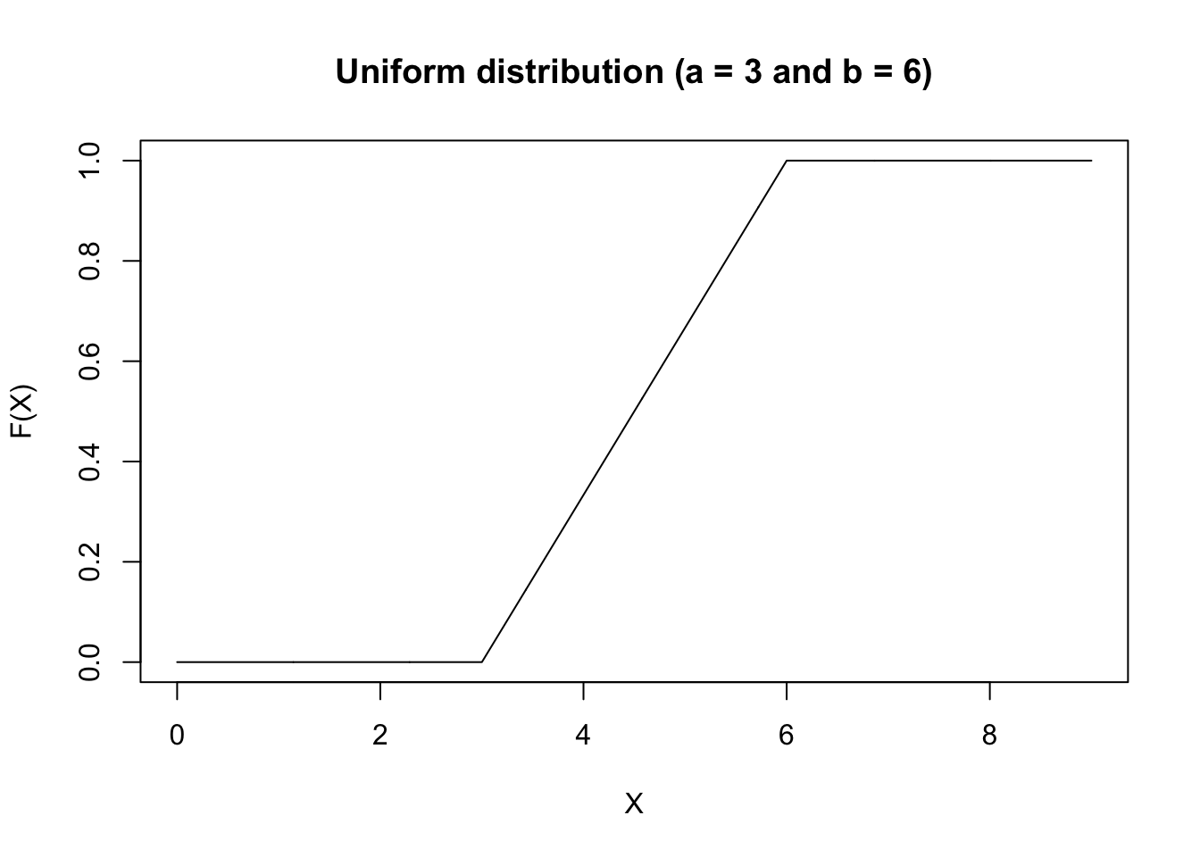
\[ \begin{align*} \begin{cases} M_X(t) = \frac{e^{bt} - e^{at}}{t(b-a)} \text{ for } t \neq 0 \\ M_X(t) = 1 \text{ for } t = 0 \\ \end{cases} \end{align*} \]

19.4 Centered Moments

\[ \mu_j = 0 \text{ if $j$ is odd} \]

\[ \mu_j = \frac{(b-a)^j}{2^j(j+1)} \text{ if $j$ is even} \]

19.5 Expected Value

\[ \text{E}(X) = \frac{a+b}{2} \]

19.6 Variance

\[ \text{V}(X) = \frac{(b-a)^2}{12} \]

19.7 Median

\[ \text{Med}(X) = \frac{a+b}{2} \]

19.8 Coefficient of Skewness

\[ g_1 = 0 \]

19.9 Coefficient of Kurtosis

\[ g_2 = \frac{9}{5} \]

19.10 Coefficient of Variation

\[ VC = \frac{1}{\sqrt{3}} \frac{b-a}{a+b} \]

19.11 Purpose

There are several random processes (such as most random sampling processes) which can be assumed to have a Uniform Distribution. The Uniform Distribution has important applications because it is used in the generation of pseudo random numbers in digital computers. In addition, it is typically used in situations when investigating the probability that an event occurs within a specified time frame while there is no systematic cause to be found (e.g. a random error occurs in an assembly line production process -- if there’s no systematic reason for the error, we assume that there is an equal probability of the error occurring between times a and b).

19.12 Example

Suppose we want to simulate the occurrence \(X\) of three mutually exclusive events \(X = A\), \(X = B\), and \(X = C\) with known probabilities that sum to 1. The event probabilities themselves are not “uniform”; instead, we use a Uniform random number generator on \([0,1]\) as a simulation mechanism. Since probabilities are conventionally bounded between 0 and 1, we set \(a = 0\) and \(b = 1\) to obtain

\[ \begin{align*} \begin{cases} \text{f}(X) = \frac{1}{1-0} \text{ for } X \in [0, 1] \\ \text{f}(X) = 0 \text{ for } X \notin [0, 1] \end{cases} \end{align*} \]

In other words, every random number that is produced by the digital computer lies between 0 and 1 with a probability of 100%. Now we can subdivide the interval \([0, 1]\) into three segments which correspond to the probabilities of each event. If, for instance, P(\(X = A\)) = 0.1, P(\(X = B\)) = 0.5, and P(\(X = C\)) = 0.4 then we can use the following rules to simulate events

\[ \begin{align*} \begin{cases} \text{P}(X = A) \text{ if } X \in [0, 0.1] \\ \text{P}(X = B) \text{ if } X \in \text{ } ]0.1, 0.6] \\ \text{P}(X = C) \text{ if } X \in \text{ } ]0.6, 1] \end{cases} \end{align*} \]

It is easy to generate random numbers from a Uniform Distribution in R. In our example we can do this as follows:

set.seed(42) # set random seed to make the result reproducible
random_events = rep("A", 100) # start with 100 events "A"
random_numbers = runif(n = 100, min = 0, max = 1) # draw 100 random numbers from U(0,1)
random_events[random_numbers > 0.1] = "B" # change all events to "B" if the random number > 0.1
random_events[random_numbers > 0.6] = "C" # change all events to "C" if the random number > 0.6
print(random_events) # print all random events
table(random_events) # frequency table
  [1] "C" "C" "B" "C" "C" "B" "C" "B" "C" "C" "B" "C" "C" "B" "B" "C" "C" "B"
 [19] "B" "B" "C" "B" "C" "C" "A" "B" "B" "C" "B" "C" "C" "C" "B" "C" "A" "C"
 [37] "A" "B" "C" "C" "B" "B" "A" "C" "B" "C" "C" "C" "C" "C" "B" "B" "B" "C"
 [55] "A" "C" "C" "B" "B" "B" "C" "C" "C" "B" "C" "B" "B" "C" "C" "B" "A" "B"
 [73] "B" "B" "B" "C" "A" "B" "B" "A" "B" "B" "B" "C" "C" "B" "B" "A" "A" "B"
 [91] "C" "A" "B" "C" "C" "C" "B" "B" "C" "C"
random_events
 A  B  C 
11 43 46 
20  Normal Distribution (Gaussian Distribution)

© 2026 Patrick Wessa. Provided as-is, without warranty.

Feedback: e-mail | Anonymous contributions: click to copy (Sats) | click to copy (XMR)

Cookie Preferences