48  Noncentral F Distribution

The Noncentral F distribution is the theoretical foundation for power analysis of ANOVA and regression F-tests. When a researcher asks how many subjects per group do I need for my ANOVA? or what power does my regression model have to detect a given $R^2$?, the answer depends on the Noncentral F distribution.

Formally, the random variate \(X\) defined for the range \(X \geq 0\), is said to have a Noncentral F Distribution (i.e. \(X \sim \text{F}(m, n, \lambda)\)) with numerator degrees of freedom \(m > 0\), denominator degrees of freedom \(n > 0\), and noncentrality parameter \(\lambda \geq 0\).

Construction. If \(U \sim \chi^2(m, \lambda)\) is a Noncentral Chi-squared variate (see Chapter 24) and \(V \sim \chi^2(n)\) is an independent central Chi-squared variate (see Chapter 23), then

\[ F = \frac{U/m}{V/n} \sim \text{F}(m, n, \lambda) \]

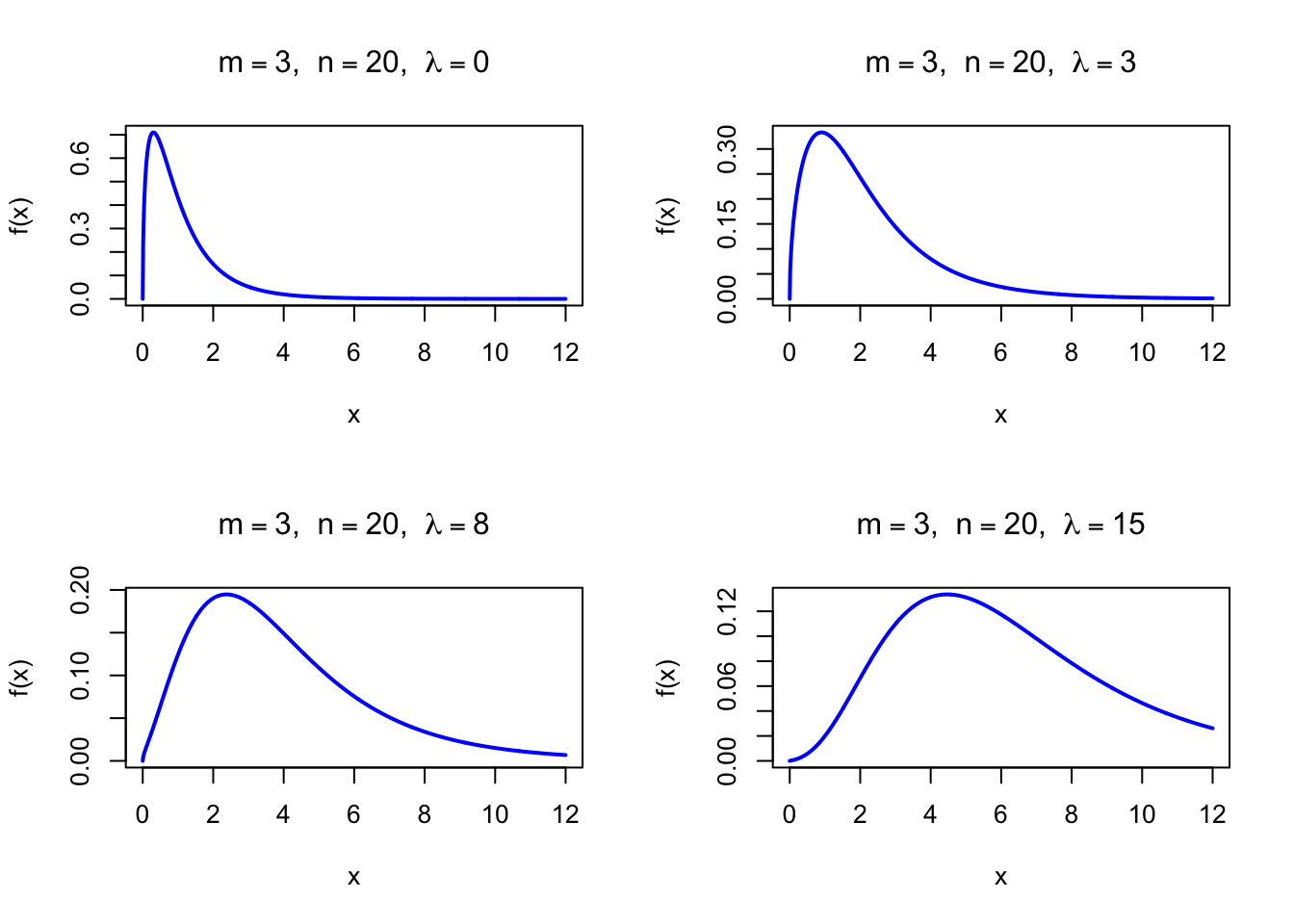
When \(\lambda = 0\), this reduces to the standard (central) Fisher F distribution (see Chapter 26). The noncentrality parameter \(\lambda\) reflects the magnitude of a true effect, shifting the distribution to the right and increasing its mean.

48.1 Probability Density Function

The PDF of the Noncentral F distribution involves an infinite series and does not have a simple closed form. It can be written as

\[ f(x) = \sum_{j=0}^{\infty} \frac{e^{-\lambda/2}(\lambda/2)^j}{j!} \cdot \frac{B\!\left(\frac{m}{2}+j, \frac{n}{2}\right)^{-1} \left(\frac{m}{n}\right)^{m/2+j} x^{m/2+j-1}}{\left(1 + \frac{m}{n}x\right)^{(m+n)/2+j}} \]

where \(B(\cdot, \cdot)\) is the Beta function. In practice, R computes the density with df(x, df1, df2, ncp).

The figure below shows the Noncentral F Probability Density Function for \(m = 3\), \(n = 20\), and several values of \(\lambda\).

par(mfrow = c(2, 2))
x <- seq(0, 12, length = 1000)

plot(x, df(x, df1 = 3, df2 = 20, ncp = 0), type = "l", lwd = 2, col = "blue",
     xlab = "x", ylab = "f(x)", main = expression(paste(m == 3, ",  ", n == 20, ",  ", lambda == 0)))

plot(x, df(x, df1 = 3, df2 = 20, ncp = 3), type = "l", lwd = 2, col = "blue",
     xlab = "x", ylab = "f(x)", main = expression(paste(m == 3, ",  ", n == 20, ",  ", lambda == 3)))

plot(x, df(x, df1 = 3, df2 = 20, ncp = 8), type = "l", lwd = 2, col = "blue",
     xlab = "x", ylab = "f(x)", main = expression(paste(m == 3, ",  ", n == 20, ",  ", lambda == 8)))

plot(x, df(x, df1 = 3, df2 = 20, ncp = 15), type = "l", lwd = 2, col = "blue",
     xlab = "x", ylab = "f(x)", main = expression(paste(m == 3, ",  ", n == 20, ",  ", lambda == 15)))

par(mfrow = c(1, 1))

Figure 48.1: Noncentral F Probability Density Function (df1 = 3, df2 = 20) for various noncentrality values

48.2 Purpose

The Noncentral F distribution is the theoretical backbone of power analysis for F-tests, including ANOVA and regression. Its primary applications include:

• ANOVA sample size planning: determining the number of observations per group needed to detect differences among \(k\) group means with desired power
• Regression power analysis: computing the power to detect a given \(R^2\) or partial \(R^2\) in linear regression
• Factorial experiment design: planning multi-factor experiments with adequate power for main effects and interactions
• Model comparison: assessing whether a study has sufficient power to distinguish between nested regression models
• Clinical trial design: justifying group sizes in multi-arm trials

Relation to the F-test. Under the null hypothesis (no group differences in ANOVA, or \(R^2 = 0\) in regression), the F statistic follows a central F distribution (\(\lambda = 0\)). Under the alternative hypothesis, it follows a Noncentral F distribution with noncentrality \(\lambda > 0\). Power is the probability that the observed F exceeds the critical value under the Noncentral F distribution.

48.3 Distribution Function

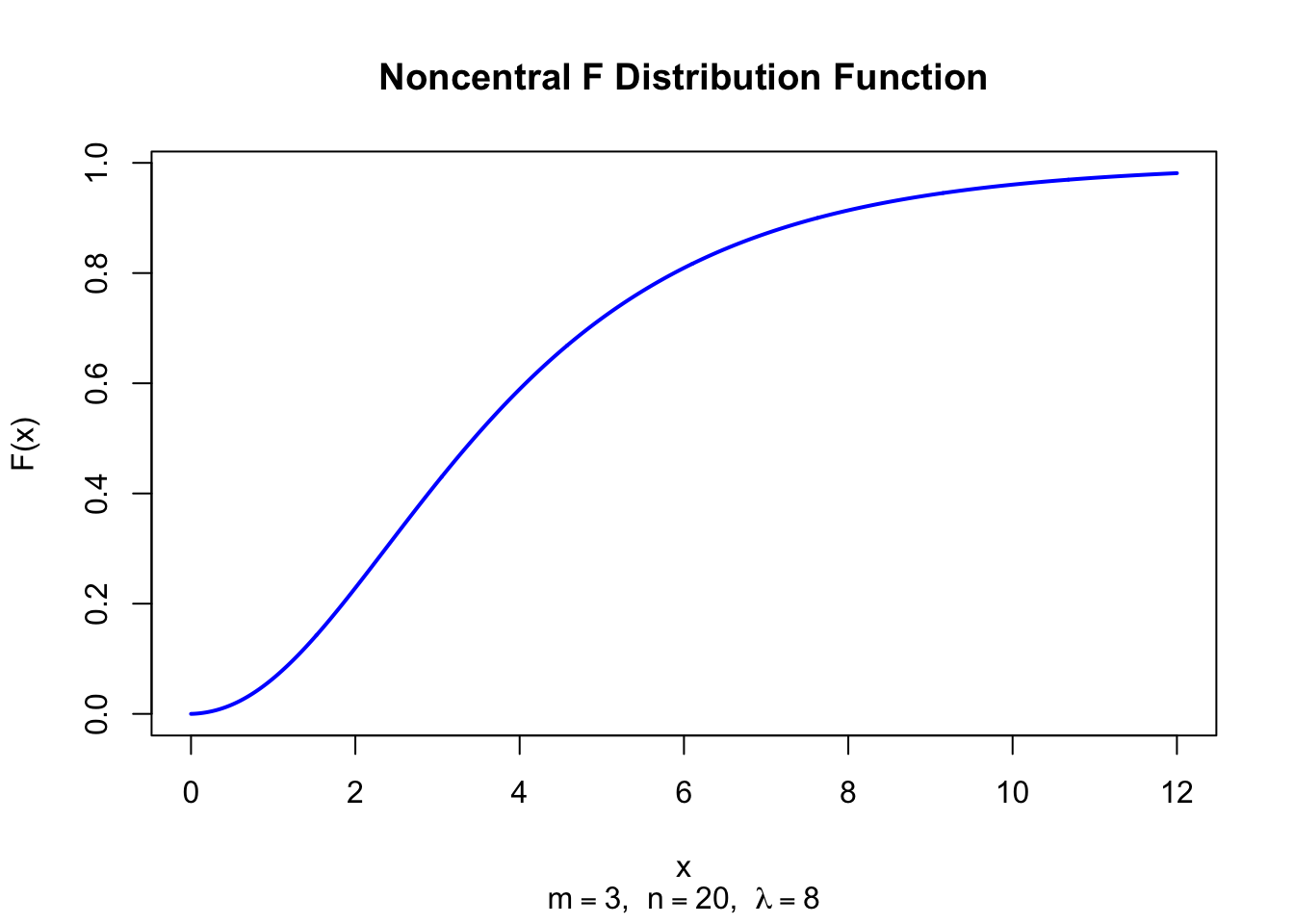
There is no elementary closed form for the CDF. It is computed numerically by pf(x, df1, df2, ncp) in R.

The figure below shows the Noncentral F Distribution Function for \(m = 3\), \(n = 20\), and \(\lambda = 8\).

x <- seq(0, 12, length = 1000)
plot(x, pf(x, df1 = 3, df2 = 20, ncp = 8), type = "l", lwd = 2, col = "blue",
     xlab = "x", ylab = "F(x)", main = "Noncentral F Distribution Function",
     sub = expression(paste(m == 3, ",  ", n == 20, ",  ", lambda == 8)))

Figure 48.2: Noncentral F Distribution Function (df1 = 3, df2 = 20, lambda = 8)

48.4 Moment Generating Function

The moment generating function of the Noncentral F distribution does not have a simple closed form.

48.5 Expected Value

\[ \text{E}(X) = \frac{n(m + \lambda)}{m(n - 2)} \quad \text{for } n > 2 \]

When \(\lambda = 0\), this reduces to \(n/(n-2)\), which is the mean of the central F distribution.

48.6 Variance

\[ \text{V}(X) = 2 \left(\frac{n}{m}\right)^2 \frac{(m + \lambda)^2 + (m + 2\lambda)(n - 2)}{(n - 2)^2 (n - 4)} \quad \text{for } n > 4 \]

48.7 Median

There is no closed-form expression for the median. It is computed numerically via qf(0.5, df1, df2, ncp) in R:

# Median for F(m = 3, n = 20, lambda = 8)
qf(0.5, df1 = 3, df2 = 20, ncp = 8)

[1] 3.443321

48.8 Mode

The mode of the Noncentral F distribution does not have a simple closed-form expression. It can be found numerically by maximizing the density function. For moderate to large noncentrality, the mode is approximately \((m + \lambda)(n - 2) / (m(n + 2))\) minus a correction term.

48.9 Coefficient of Skewness

The Noncentral F distribution is always right-skewed. The skewness depends on all three parameters (\(m\), \(n\), \(\lambda\)) and requires \(n > 6\) for existence. As the noncentrality \(\lambda\) increases, the skewness changes in a complex way. When \(\lambda = 0\), the skewness reduces to that of the central F distribution.

48.10 Coefficient of Kurtosis

The kurtosis of the Noncentral F distribution depends on \(m\), \(n\), and \(\lambda\), and requires \(n > 8\) for existence. The distribution is leptokurtic (kurtosis exceeds 3), with heavier tails than the Normal distribution. As \(n \to \infty\), the kurtosis decreases toward values closer to the Normal benchmark.

48.11 Parameter Estimation

Like the Noncentral t distribution, the Noncentral F distribution is not typically fitted to data via classical parameter estimation. Instead, the noncentrality parameter \(\lambda\) is determined from the experimental design:

• One-way ANOVA (\(k\) groups, each with \(n\) observations): \(\lambda = k \cdot n \cdot f^2\), where \(f\) is Cohen’s \(f\) effect size defined as \(f = \sigma_{\text{between}} / \sigma_{\text{within}}\)
• Regression (\(p\) predictors, \(N\) total observations): \(\lambda = \frac{N \cdot R^2}{1 - R^2}\) for the overall F-test of the model
• Partial F-test (testing \(q\) additional predictors): \(\lambda = (N - p_{\text{reduced}})\,f^2_{\text{partial}}\) where \(f^2_{\text{partial}} = (R^2_{\text{full}} - R^2_{\text{reduced}}) / (1 - R^2_{\text{full}})\)

Cohen’s conventional benchmarks for \(f\) are: small = 0.10, medium = 0.25, large = 0.40.

48.12 R Module

48.12.1 RFC

The Noncentral F Distribution module is available in RFC under the menu “Distributions / Noncentral F Distribution”.

48.12.2 Direct app link

• https://shiny.wessa.net/ncfdist/

48.12.3 R Code

The following code demonstrates Noncentral F probability calculations:

# Probability density function: f(x)
df(x = 3, df1 = 3, df2 = 20, ncp = 8)

# Distribution function: P(X <= x)
pf(q = 3, df1 = 3, df2 = 20, ncp = 8)

# Quantile function: find x such that P(X <= x) = p
qf(p = 0.95, df1 = 3, df2 = 20, ncp = 8)

# Generate random Noncentral F numbers
set.seed(42)
rf(n = 10, df1 = 3, df2 = 20, ncp = 8)

[1] 0.185492
[1] 0.4207864
[1] 9.388105
 [1]  5.123445  4.143252  4.889171  4.394841 20.075338  5.881126 16.961353
 [8]  2.524019  2.606690  5.403320

48.13 Example

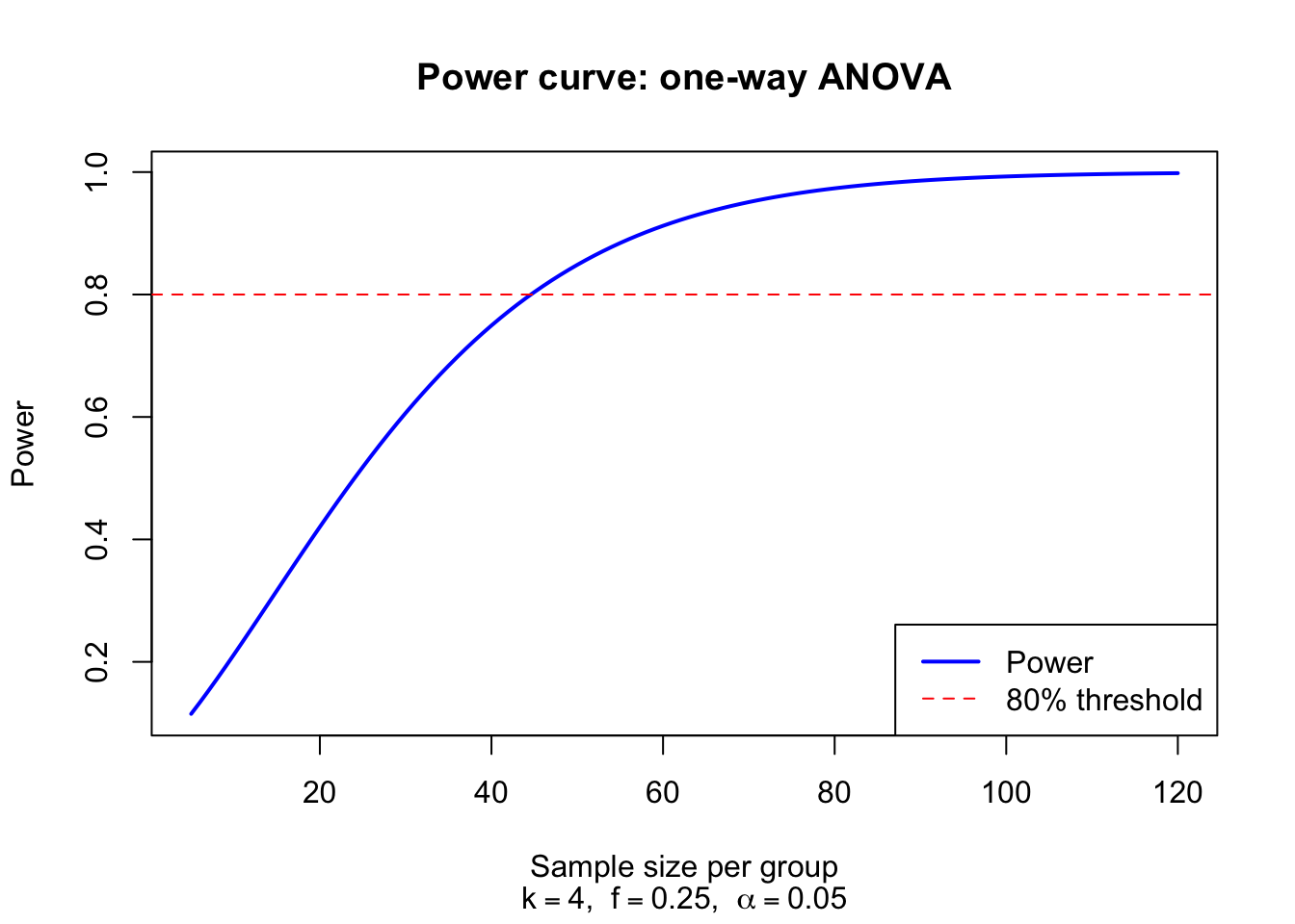
A psychologist plans a one-way ANOVA comparing \(k = 4\) treatment groups. Based on prior studies, a medium effect (\(f = 0.25\)) is expected. Using \(\alpha = 0.05\), how many subjects per group are needed for 80% power?

The noncentrality parameter for a one-way ANOVA is \(\lambda = k \cdot n \cdot f^2\), the numerator degrees of freedom are \(m = k - 1 = 3\), and the denominator degrees of freedom are \(n_{\text{denom}} = k(n - 1)\). We compute power for various group sizes:

k     <- 4       # number of groups
f     <- 0.25    # Cohen's f (medium effect)
alpha <- 0.05    # significance level

# Compute power for group sizes from 10 to 80
n_per_group <- seq(10, 80, by = 5)
power       <- numeric(length(n_per_group))

for (i in seq_along(n_per_group)) {
  n_g    <- n_per_group[i]
  df1    <- k - 1
  df2    <- k * (n_g - 1)
  lambda <- k * n_g * f^2
  f_crit <- qf(1 - alpha, df1 = df1, df2 = df2)
  power[i] <- 1 - pf(f_crit, df1 = df1, df2 = df2, ncp = lambda)
}

result <- data.frame(n_per_group = n_per_group,
                     N_total = k * n_per_group,
                     lambda = k * n_per_group * f^2,
                     power = round(power, 4))
print(result)

# Find minimum group size for 80% power
n_required <- n_per_group[which(power >= 0.80)[1]]
cat("\nMinimum per-group sample size for 80% power:", n_required, "\n")
cat("Total sample size:", k * n_required, "\n")

   n_per_group N_total lambda  power
1           10      40   2.50 0.2122
2           15      60   3.75 0.3166
3           20      80   5.00 0.4204
4           25     100   6.25 0.5182
5           30     120   7.50 0.6065
6           35     140   8.75 0.6837
7           40     160  10.00 0.7494
8           45     180  11.25 0.8040
9           50     200  12.50 0.8485
10          55     220  13.75 0.8841
11          60     240  15.00 0.9122
12          65     260  16.25 0.9341
13          70     280  17.50 0.9510
14          75     300  18.75 0.9638
15          80     320  20.00 0.9735

Minimum per-group sample size for 80% power: 45 
Total sample size: 180 

k     <- 4
f     <- 0.25
alpha <- 0.05
n_per_group <- seq(5, 120, by = 1)
power       <- numeric(length(n_per_group))
for (i in seq_along(n_per_group)) {
  n_g    <- n_per_group[i]
  df1    <- k - 1
  df2    <- k * (n_g - 1)
  lambda <- k * n_g * f^2
  f_crit <- qf(1 - alpha, df1 = df1, df2 = df2)
  power[i] <- 1 - pf(f_crit, df1 = df1, df2 = df2, ncp = lambda)
}
plot(n_per_group, power, type = "l", lwd = 2, col = "blue",
     xlab = "Sample size per group", ylab = "Power",
     main = "Power curve: one-way ANOVA",
     sub = expression(paste(k == 4, ",  ", f == 0.25, ",  ", alpha == 0.05)))
abline(h = 0.80, lty = 2, col = "red")
legend("bottomright", legend = c("Power", "80% threshold"),
       col = c("blue", "red"), lty = c(1, 2), lwd = c(2, 1))

Figure 48.3: Power curve for one-way ANOVA (k = 4 groups, f = 0.25, alpha = 0.05)

You can reproduce the ANOVA calculation interactively using the Noncentral F Distribution app:

Interactive Shiny app (click to load).

Open in new tab

A second common application is regression power analysis. Suppose a researcher plans a regression with \(p = 5\) predictors and expects \(R^2 = 0.13\) (medium effect). How many observations are needed for 80% power?

p     <- 5       # number of predictors
R2    <- 0.13    # expected R-squared (medium effect)
alpha <- 0.05

N_vals <- seq(30, 200, by = 5)
power  <- numeric(length(N_vals))

for (i in seq_along(N_vals)) {
  N      <- N_vals[i]
  df1    <- p
  df2    <- N - p - 1
  lambda <- N * R2 / (1 - R2)
  f_crit <- qf(1 - alpha, df1 = df1, df2 = df2)
  power[i] <- 1 - pf(f_crit, df1 = df1, df2 = df2, ncp = lambda)
}

result <- data.frame(N = N_vals, lambda = round(N_vals * R2 / (1 - R2), 2),
                     power = round(power, 4))
print(result)

# Find the exact minimum N by checking every feasible sample size
N_search <- seq(p + 2, 200, by = 1)
power_search <- numeric(length(N_search))

for (i in seq_along(N_search)) {
  N      <- N_search[i]
  df1    <- p
  df2    <- N - p - 1
  lambda <- N * R2 / (1 - R2)
  f_crit <- qf(1 - alpha, df1 = df1, df2 = df2)
  power_search[i] <- 1 - pf(f_crit, df1 = df1, df2 = df2, ncp = lambda)
}

N_required <- N_search[which(power_search >= 0.80)[1]]
cat("\nMinimum total sample size for 80% power:", N_required, "\n")

     N lambda  power
1   30   4.48 0.2641
2   35   5.23 0.3171
3   40   5.98 0.3704
4   45   6.72 0.4231
5   50   7.47 0.4745
6   55   8.22 0.5240
7   60   8.97 0.5710
8   65   9.71 0.6154
9   70  10.46 0.6568
10  75  11.21 0.6951
11  80  11.95 0.7303
12  85  12.70 0.7625
13  90  13.45 0.7916
14  95  14.20 0.8178
15 100  14.94 0.8414
16 105  15.69 0.8623
17 110  16.44 0.8809
18 115  17.18 0.8973
19 120  17.93 0.9117
20 125  18.68 0.9243
21 130  19.43 0.9353
22 135  20.17 0.9448
23 140  20.92 0.9531
24 145  21.67 0.9602
25 150  22.41 0.9663
26 155  23.16 0.9716
27 160  23.91 0.9761
28 165  24.66 0.9799
29 170  25.40 0.9831
30 175  26.15 0.9859
31 180  26.90 0.9882
32 185  27.64 0.9902
33 190  28.39 0.9918
34 195  29.14 0.9932
35 200  29.89 0.9944

Minimum total sample size for 80% power: 92 

You can reproduce the regression calculation interactively using the Noncentral F Distribution app:

Interactive Shiny app (click to load).

Open in new tab

48.14 Random Number Generator

Random variates from the Noncentral F distribution can be generated directly from its construction. If \(U \sim \chi^2(m, \lambda)\) (Noncentral Chi-squared) and \(V \sim \chi^2(n)\) (central Chi-squared) are independent, then \(F = (U/m)/(V/n)\) follows \(\text{F}(m, n, \lambda)\).

In R, a Noncentral Chi-squared variate \(\chi^2(m, \lambda)\) can be generated as the sum of \(m - 1\) independent squared standard normal variates plus one squared \(\text{N}(\sqrt{\lambda}, 1)\) variate, or directly via rchisq(1, df = m, ncp = lambda).

set.seed(123)
N      <- 1000
m      <- 3
n      <- 20
lambda <- 8

# Construction method
u <- rchisq(N, df = m, ncp = lambda)
v <- rchisq(N, df = n)
x_construct <- (u / m) / (v / n)

# Built-in function
x_rf <- rf(N, df1 = m, df2 = n, ncp = lambda)

cat("Construction: mean =", round(mean(x_construct), 4),
    "  var =", round(var(x_construct), 4), "\n")
cat("rf():         mean =", round(mean(x_rf), 4),
    "  var =", round(var(x_rf), 4), "\n")

# Theoretical mean (requires n > 2)
E_theory <- n * (m + lambda) / (m * (n - 2))
cat("Theoretical:  mean =", round(E_theory, 4), "\n")

Construction: mean = 3.9133   var = 6.7732 
rf():         mean = 3.862   var = 7.5764 
Theoretical:  mean = 4.0741 

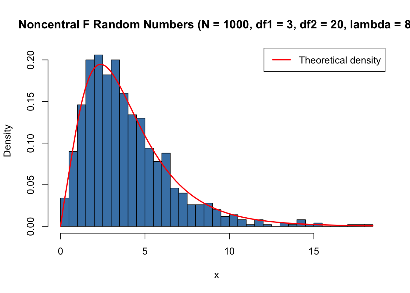
set.seed(123)
x <- rf(1000, df1 = 3, df2 = 20, ncp = 8)
hist(x, breaks = 40, col = "steelblue", freq = FALSE,
     xlab = "x", main = "Noncentral F Random Numbers (N = 1000, df1 = 3, df2 = 20, lambda = 8)")
curve(df(x, df1 = 3, df2 = 20, ncp = 8), add = TRUE, col = "red", lwd = 2)
legend("topright", legend = "Theoretical density", col = "red", lwd = 2)

Figure 48.4: Histogram of simulated Noncentral F random numbers (N = 1000, df1 = 3, df2 = 20, lambda = 8)

Interactive Shiny app (click to load).

Open in new tab

48.15 Property 1: Noncentrality and Power for ANOVA

Under the null hypothesis of equal population means, the ANOVA F statistic follows a central \(\text{F}(k-1, N-k)\). Under the alternative, it follows \(\text{F}(k-1, N-k, \lambda)\) where

\[ \lambda = k \cdot n \cdot f^2 = \sum_{j=1}^{k} n_j \left(\frac{\mu_j - \bar{\mu}}{\sigma}\right)^2 \]

Power is the probability that the observed F exceeds the critical value:

\[ \text{Power} = \text{P}\!\left(F > F_{\alpha, m, n}\right) \quad \text{where } F \sim \text{F}(m, n, \lambda) \]

As \(\lambda\) increases (larger effect or more observations per group), the Noncentral F density shifts to the right and more of its area falls beyond the critical value.

48.16 Property 2: Noncentrality Formulas for Regression

For testing the overall significance of a regression model with \(p\) predictors and \(N\) observations:

\[ \lambda = \frac{N R^2}{1 - R^2} \]

For testing \(q\) additional predictors in a partial F-test:

\[ \lambda = (N - p_{\text{reduced}})\,\frac{R^2_{\text{full}} - R^2_{\text{reduced}}}{1 - R^2_{\text{full}}} \]

These formulas directly connect effect sizes in regression to the noncentrality parameter.

48.17 Property 3: Convergence to Noncentral Chi-squared

As \(n \to \infty\), the scaled Noncentral F distribution converges to a scaled Noncentral Chi-squared:

\[ m \cdot \text{F}(m, n, \lambda) \xrightarrow{d} \chi^2(m, \lambda) \quad \text{as } n \to \infty \]

This follows from \(V/n \xrightarrow{p} 1\) as \(n \to \infty\).

48.18 Property 4: Reciprocal Property

Unlike the central F distribution, the reciprocal of a Noncentral F variate does not follow a Noncentral F distribution. Therefore, the reciprocal symmetry of the central F (see Chapter 26) does not extend to the noncentral case.

48.19 Related Distributions 1: Central F as Special Case

The Fisher F distribution is the Noncentral F distribution with noncentrality parameter \(\lambda = 0\) (see Chapter 26):

\[ \text{F}(m, n, 0) = \text{F}(m, n) \]

48.20 Related Distributions 2: Link with the Noncentral t Distribution

The square of a Noncentral t variate gives a Noncentral F variate with \(m = 1\) (see Chapter 47):

\[ T^2 \sim \text{F}(1, n, \delta^2) \quad \text{where } T \sim \text{t}(n, \delta) \]

This means that power analysis for a two-sided t-test (with noncentrality \(\delta\)) is equivalent to power analysis for an F-test with \(m = 1\) and noncentrality \(\lambda = \delta^2\).

48.21 Related Distributions 3: Noncentral Chi-squared Connection

The Noncentral F distribution is constructed from the ratio of a Noncentral Chi-squared variate and an independent central Chi-squared variate (see Chapter 24). As \(n \to \infty\), the denominator converges to 1, and the Noncentral F converges to a scaled Noncentral Chi-squared.

48.22 Related Distributions 4: Beta Connection

The Noncentral F distribution is related to the Noncentral Beta distribution in the same way the central F is related to the Beta distribution (see Chapter 30). If \(X \sim \text{F}(m, n, \lambda)\), then \(Y = \frac{mX/n}{1 + mX/n}\) follows a Noncentral Beta distribution.