• Descriptive
    • Moments
    • Concentration
    • Central Tendency
    • Variability
    • Stem-and-Leaf Plot
    • Histogram & Frequency Table
    • Data Quality Forensics
    • Conditional EDA
    • Quantiles
    • Kernel Density Estimation
    • Normal QQ Plot
    • Bootstrap Plot

    • Multivariate Descriptive Statistics
  • Distributions
    • Binomial Probabilities
    • Geometric Probabilities
    • Negative Binomial Probabilities
    • Hypergeometric Probabilities
    • Multinomial Probabilities
    • Dirichlet
    • Poisson Probabilities

    • Exponential
    • Gamma
    • Erlang
    • Weibull
    • Rayleigh
    • Maxwell-Boltzmann
    • Lognormal
    • Pareto
    • Inverse Gamma
    • Inverse Chi-Square

    • Beta
    • Power
    • Beta Prime (Inv. Beta)
    • Triangular

    • Normal (area)
    • Logistic
    • Laplace
    • Cauchy (standard)
    • Cauchy (location-scale)
    • Gumbel
    • Fréchet
    • Generalized Extreme Value

    • Normal RNG
    • ML Fitting
    • Tukey Lambda PPCC
    • Box-Cox Normality Plot
    • Noncentral t
    • Noncentral F
    • Sample Correlation r

    • Empirical Tests
  • Hypotheses
    • Theoretical Aspects of Hypothesis Testing
    • Bayesian Inference
    • Minimum Sample Size

    • Empirical Tests
    • Multivariate (pair-wise) Testing
  • Models
    • Manual Model Building
    • Guided Model Building
  • Time Series
    • Time Series Plot
    • Decomposition
    • Exponential Smoothing

    • Blocked Bootstrap Plot
    • Mean Plot
    • (P)ACF
    • VRM
    • Standard Deviation-Mean Plot
    • Spectral Analysis
    • ARIMA

    • Cross Correlation Function
    • Granger Causality
  1. Descriptive Statistics & Exploratory Data Analysis
  2. 92  (Partial) Autocorrelation Function
  • Preface
  • Getting Started
    • 1  Introduction
    • 2  Why Do We Need Innovative Technology?
    • 3  Basic Definitions
    • 4  The Big Picture: Why We Analyze Data
  • Introduction to Probability
    • 5  Definitions of Probability
    • 6  Jeffreys’ axiom system
    • 7  Bayes’ Theorem
    • 8  Sensitivity and Specificity
    • 9  Naive Bayes Classifier
    • 10  Law of Large Numbers

    • 11  Problems
  • Probability Distributions
    • 12  Bernoulli Distribution
    • 13  Binomial Distribution
    • 14  Geometric Distribution
    • 15  Negative Binomial Distribution
    • 16  Hypergeometric Distribution
    • 17  Multinomial Distribution
    • 18  Poisson Distribution

    • 19  Uniform Distribution (Rectangular Distribution)
    • 20  Normal Distribution (Gaussian Distribution)
    • 21  Gaussian Naive Bayes Classifier
    • 22  Chi Distribution
    • 23  Chi-squared Distribution (1 parameter)
    • 24  Chi-squared Distribution (2 parameters)
    • 25  Student t-Distribution
    • 26  Fisher F-Distribution
    • 27  Exponential Distribution
    • 28  Lognormal Distribution
    • 29  Gamma Distribution
    • 30  Beta Distribution
    • 31  Weibull Distribution
    • 32  Pareto Distribution
    • 33  Inverse Gamma Distribution
    • 34  Rayleigh Distribution
    • 35  Erlang Distribution
    • 36  Logistic Distribution
    • 37  Laplace Distribution
    • 38  Gumbel Distribution
    • 39  Cauchy Distribution
    • 40  Triangular Distribution
    • 41  Power Distribution
    • 42  Beta Prime Distribution
    • 43  Sample Correlation Distribution
    • 44  Dirichlet Distribution
    • 45  Generalized Extreme Value (GEV) Distribution
    • 46  Frechet Distribution
    • 47  Noncentral t Distribution
    • 48  Noncentral F Distribution
    • 49  Inverse Chi-Squared Distribution
    • 50  Maxwell-Boltzmann Distribution
    • 51  Distribution Relationship Map

    • 52  Problems
  • Descriptive Statistics & Exploratory Data Analysis
    • 53  Types of Data
    • 54  Datasheets

    • 55  Frequency Plot (Bar Plot)
    • 56  Frequency Table
    • 57  Contingency Table
    • 58  Binomial Classification Metrics
    • 59  Confusion Matrix
    • 60  ROC Analysis

    • 61  Stem-and-Leaf Plot
    • 62  Histogram
    • 63  Data Quality Forensics
    • 64  Quantiles
    • 65  Central Tendency
    • 66  Variability
    • 67  Skewness & Kurtosis
    • 68  Concentration
    • 69  Notched Boxplot
    • 70  Scatterplot
    • 71  Pearson Correlation
    • 72  Rank Correlation
    • 73  Partial Pearson Correlation
    • 74  Simple Linear Regression
    • 75  Moments
    • 76  Quantile-Quantile Plot (QQ Plot)
    • 77  Normal Probability Plot
    • 78  Probability Plot Correlation Coefficient Plot (PPCC Plot)
    • 79  Box-Cox Normality Plot
    • 80  Kernel Density Estimation
    • 81  Bivariate Kernel Density Plot
    • 82  Conditional EDA: Panel Diagnostics
    • 83  Bootstrap Plot (Central Tendency)
    • 84  Survey Scores Rank Order Comparison
    • 85  Cronbach Alpha

    • 86  Equi-distant Time Series
    • 87  Time Series Plot (Run Sequence Plot)
    • 88  Mean Plot
    • 89  Blocked Bootstrap Plot (Central Tendency)
    • 90  Standard Deviation-Mean Plot
    • 91  Variance Reduction Matrix
    • 92  (Partial) Autocorrelation Function
    • 93  Periodogram & Cumulative Periodogram

    • 94  Problems
  • Hypothesis Testing
    • 95  Normal Distributions revisited
    • 96  The Population
    • 97  The Sample
    • 98  The One-Sided Hypothesis Test
    • 99  The Two-Sided Hypothesis Test
    • 100  When to use a one-sided or two-sided test?
    • 101  What if \(\sigma\) is unknown?
    • 102  The Central Limit Theorem (revisited)
    • 103  Statistical Test of the Population Mean with known Variance
    • 104  Statistical Test of the Population Mean with unknown Variance
    • 105  Statistical Test of the Variance
    • 106  Statistical Test of the Population Proportion
    • 107  Statistical Test of the Standard Deviation \(\sigma\)
    • 108  Statistical Test of the difference between Means -- Independent/Unpaired Samples
    • 109  Statistical Test of the difference between Means -- Dependent/Paired Samples
    • 110  Statistical Test of the difference between Variances -- Independent/Unpaired Samples

    • 111  Hypothesis Testing for Research Purposes
    • 112  Decision Thresholds, Alpha, and Confidence Levels
    • 113  Bayesian Inference for Decision-Making
    • 114  One Sample t-Test
    • 115  Skewness & Kurtosis Tests
    • 116  Paired Two Sample t-Test
    • 117  Wilcoxon Signed-Rank Test
    • 118  Unpaired Two Sample t-Test
    • 119  Unpaired Two Sample Welch Test
    • 120  Two One-Sided Tests (TOST) for Equivalence
    • 121  Mann-Whitney U test (Wilcoxon Rank-Sum Test)
    • 122  Bayesian Two Sample Test
    • 123  Median Test based on Notched Boxplots
    • 124  Chi-Squared Tests for Count Data
    • 125  Kolmogorov-Smirnov Test
    • 126  One Way Analysis of Variance (1-way ANOVA)
    • 127  Kruskal-Wallis Test
    • 128  Two Way Analysis of Variance (2-way ANOVA)
    • 129  Repeated Measures ANOVA
    • 130  Friedman Test
    • 131  Testing Correlations
    • 132  A Note on Causality

    • 133  Problems
  • Regression Models
    • 134  Simple Linear Regression Model (SLRM)
    • 135  Multiple Linear Regression Model (MLRM)
    • 136  Logistic Regression
    • 137  Generalized Linear Models
    • 138  Multinomial and Ordinal Logistic Regression
    • 139  Cox Proportional Hazards Regression
    • 140  Conditional Inference Trees
    • 141  Leaf Diagnostics for Conditional Inference Trees
    • 142  Conditional Random Forests
    • 143  Hypothesis Testing with Linear Regression Models (from a Practical Point of View)

    • 144  Problems
  • Introduction to Time Series Analysis
    • 145  Case: the Market of Health and Personal Care Products
    • 146  Decomposition of Time Series
    • 147  Ad hoc Forecasting of Time Series
  • Box-Jenkins Analysis
    • 148  Introduction to Box-Jenkins Analysis
    • 149  Theoretical Concepts
    • 150  Stationarity
    • 151  Identifying ARMA parameters
    • 152  Estimating ARMA Parameters and Residual Diagnostics
    • 153  Forecasting with ARIMA models
    • 154  Intervention Analysis
    • 155  Cross-Correlation Function
    • 156  Transfer Function Noise Models
    • 157  General-to-Specific Modeling
  • Model Building Strategies
    • 158  Introduction to Model Building Strategies
    • 159  Manual Model Building
    • 160  Model Validation
    • 161  Regularization Methods
    • 162  Hyperparameter Optimization Strategies
    • 163  Guided Model Building in Practice
    • 164  Diagnostics, Revision, and Guided Forecasting
    • 165  Leakage, Target Encoding, and Robust Regression
  • References
  • Appendices
    • Appendices
    • A  Method Selection Guide
    • B  Presentations and Teaching Materials
    • C  R Language Concepts for Statistical Computing
    • D  Matrix Algebra
    • E  Standard Normal Table (Gaussian Table)
    • F  Critical values of Student’s \(t\) distribution with \(\nu\) degrees of freedom
    • G  Upper-tail critical values of the \(\chi^2\)-distribution with \(\nu\) degrees of freedom
    • H  Lower-tail critical values of the \(\chi^2\)-distribution with \(\nu\) degrees of freedom

Table of contents

  • 92.1 Definition
    • 92.1.1 Horizontal axis
    • 92.1.2 Vertical axis
  • 92.2 R Module
    • 92.2.1 Public website
    • 92.2.2 RFC
  • 92.3 Purpose
  • 92.4 Pros & Cons
    • 92.4.1 Pros
    • 92.4.2 Cons
  • 92.5 Example
  • 92.6 Task
  1. Descriptive Statistics & Exploratory Data Analysis
  2. 92  (Partial) Autocorrelation Function

92  (Partial) Autocorrelation Function

92.1 Definition

The Autocorrelation Function (ACF) of a time series \(Y_t\) relates sequential correlations (on the y-axis) \(\rho_k = \rho(Y_t, Y_{t-k})\) for \(k = 1, 2, …, K\) to the time lag \(k\) (on the x-axis). Often this is presented in graphical form because it allows to quickly detect patterns that are typical of the dynamical properties of the underlying time series. Note that the time lag \(k\) is sometimes called the “order” of autocorrelation.

The sample autocorrelations are computed by the formula

\[ \hat{\rho}_k = \frac{\overset{T}{\underset{t=k+1}\sum} \left( (Y_t - \bar{Y})(Y_{t-k} - \bar{Y}) \right) }{\overset{T}{\underset{t=1}\sum} \left(Y_t - \bar{Y} \right)^2} \]

with

\[ \bar{Y} = \frac{1}{T} \overset{T}{\underset{t=1}\sum} Y_t \]

The 95% Confidence Intervals (of individual autocorrelation coefficients) are displayed as two horizontal lines, based on the approximated standard deviation \(\sigma_{\rho_k} \simeq \tfrac{1}{\sqrt{T}}\) (Bartlett 1946). These bands assume a white-noise null hypothesis (approximately i.i.d. observations/residuals); if that assumption is violated, they are only approximate and may be anti-conservative.

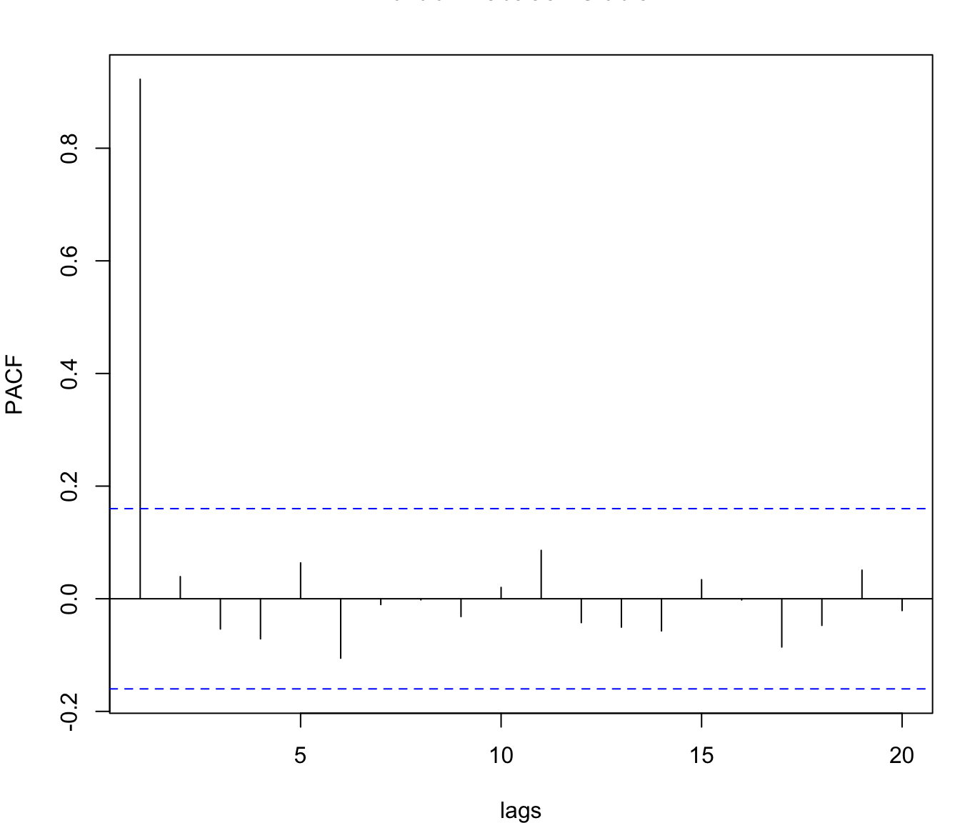
The Partial Autocorrelation Function (PACF) at lag \(k\) is the correlation between \(Y_t\) and \(Y_{t-k}\) after removing the linear effects of the intermediate lags \(Y_{t-1},\ldots,Y_{t-k+1}\). In practice, PACF isolates the direct lag-\(k\) relationship that is not explained by shorter lags.

92.1.1 Horizontal axis

The horizontal axis displays the time lag \(k\).

92.1.2 Vertical axis

The vertical axis represents the autocorrelation coefficients \(\hat{\rho}_k\).

92.2 R Module

92.2.1 Public website

The (Partial) Autocorrelation Function is available on the public website:

  • https://compute.wessa.net/rwasp_autocorrelation.wasp

92.2.2 RFC

The (Partial) Autocorrelation Function is also available in RFC (when using the default profile) under the “Time Series / (P)ACF” menu item.

To compute the (Partial) Autocorrelation Function on your local machine, the following script can be used in the R console:

par(mar = c(4, 4, 2, 1))
x <- 100 + cumsum(rnorm(150))
summary(x)
par1 = 20 #number of time lags
par2 = 1 #Box-Cox transformation parameter
par3 = 0 #degree of non-seasonal differencing
par4 = 0 #degree of seasonal differencing
par5 = 12 #seasonality
par6 = 'White Noise' #type of confidence interval
par7 = 0.95 #confidence interval
par8 = ''
if (par1 == 'Default') {
  par1 = 10*log10(length(x))
} else {
  par1 <- as.numeric(par1)
}
if (par6 == 'White Noise') par6 <- 'white' else par6 <- 'ma'
if (par8 != '') par8 <- as.numeric(par8)
ox <- x
if (par8 == '') {
  if (par2 == 0) {
    x <- log(x)
  } else {
    x <- (x ^ par2 - 1) / par2
  }
} else {
  x <- log(x,base=par8)
}
if (par3 > 0) x <- diff(x,lag=1,difference=par3)
if (par4 > 0) x <- diff(x,lag=par5,difference=par4)
op <- par(mfrow=c(2,1))
plot(ox,type='l',main='Original Time Series',xlab='time',ylab='value')
if (par8=='') {
  mytitle <- paste('Working Time Series (lambda=',par2,', d=',par3,', D=',par4,')',sep='')
  mysub <- paste('(lambda=',par2,', d=',par3,', D=',par4,', CI=', par7, ', CI type=',par6,')',sep='')
} else {
  mytitle <- paste('Working Time Series (base=',par8,', d=',par3,', D=',par4,')',sep='')
  mysub <- paste('(base=',par8,', d=',par3,', D=',par4,', CI=', par7, ', CI type=',par6,')',sep='')
}
plot(x,type='l', main=mytitle,xlab='time',ylab='value')

par(op)
racf <- acf(x, par1, main='Autocorrelation', xlab='time lag', ylab='ACF', ci.type=par6, ci=par7, sub=mysub)

rpacf <- pacf(x,par1,main='Partial Autocorrelation',xlab='lags',ylab='PACF',sub=mysub)

df = data.frame(k = 0:par1, ACF = c(racf$acf), PACF = c(NA, rpacf$acf))
print(df)
   Min. 1st Qu.  Median    Mean 3rd Qu.    Max. 
  94.62   97.90   99.11   99.65  101.75  105.40 
    k        ACF         PACF
1   0 1.00000000           NA
2   1 0.92244505  0.922445055
3   2 0.85676937  0.039333913
4   3 0.78752943 -0.053673907
5   4 0.71391579 -0.071177562
6   5 0.65667202  0.063758993
7   6 0.58662679 -0.105598022
8   7 0.52356094 -0.010324303
9   8 0.46587407 -0.001963130
10  9 0.40683487 -0.031680865
11 10 0.35960417  0.020227141
12 11 0.32727544  0.085935071
13 12 0.29117677 -0.042410444
14 13 0.25451010 -0.050473886
15 14 0.21285908 -0.057095254
16 15 0.17999680  0.033860294
17 16 0.15224966 -0.002072882
18 17 0.11425926 -0.085751888
19 18 0.07636231 -0.047282307
20 19 0.04828137  0.050807506
21 20 0.01878635 -0.020996578

To compute the (Partial) Autocorrelation Function, the R code uses the standard acf and pacf functions to compute the analysis.

92.3 Purpose

In practice the ACF can be used to:

  • describe/summarize autocorrelation at various orders
  • identify non-seasonal and seasonal trends
  • identify various types of typical patterns that correspond to well-known forecasting models
  • check the independence assumption of the residuals of regression and forecasting models

92.4 Pros & Cons

92.4.1 Pros

The (Partial) Autocorrelation Function has the following advantages:

  • It is relatively easy to interpret and provide a lot of information about the serial correlation of a time series.
  • It can be computed with many software packages (even though one should be careful when using spreadsheets because they do not take empty cells that occur in lagged time series into account properly).
  • The combination of Partial and (ordinary) Autocorrelation Functions allows one to identify how the time series model should be specified (Box and Jenkins 1970).
  • It allows one to check an important assumption of residuals (prediction errors).

92.4.2 Cons

The (Partial) Autocorrelation Function has the following disadvantages:

  • It is sensitive to outliers.
  • The confidence intervals are not always computed correctly in statistical software. There are (at least) two types of confidence intervals: one for testing whether residuals contain autocorrelation1 and another which should be used to identify the autocorrelation structure of the time series model2.

92.5 Example

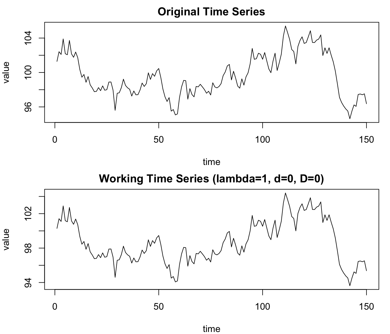
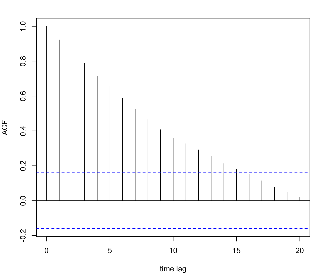
Let us consider the Airline Data and apply the ACF analysis. In a first stage we compute the ACF without any differencing, i.e. \(d = D = 0\) (these parameters were introduced in Section 91.1). The analysis shows the ACF for the original time series and exhibits a pattern which is typical for time series with a non-seasonal trend and strong seasonality:

  • The coefficients of the ACF are positive and slowly decreasing.
  • The seasonal coefficients, i.e. \(\rho_{12}, \rho_{24}, \rho_{36}, ...\) are positive and slowly decreasing too.
Interactive Shiny app (click to load).
Open in new tab

In the next step we set \(d = 1\) in order to apply non-seasonal differencing (the other parameter is not changed, \(D = 0\)). When we recompute the ACF (with \(d=1\)) then an entirely different pattern is observed, as is shown in the R module where the long-run trend pattern has disappeared. Only the seasonal Autocorrelation coefficients are still clearly positive and slowly decreasing, indicating the presence of a strong, seasonal pattern.

Finally we set \(d = D = 1\) to apply ordinary and seasonal differencing before recomputing the ACF. The R module shows that the combined differencing procedures eliminate the trend and the seasonal pattern. We can see this in the ACF because it does not exhibit the typical seasonality pattern anymore.

In later chapters, this information will be used to build a practical forecasting model for the Airline time series.

92.6 Task

Based on the ACF, examine the monthly time series of Divorces and determine whether or not there is a long-run trend and seasonality.

Bartlett, M. S. 1946. “On the Theoretical Specification and Sampling Properties of Autocorrelated Time-Series.” Journal of the Royal Statistical Society. Series B (Methodological) 8 (1): 27–41.
Box, George E. P., and Gwilym M. Jenkins. 1970. Time Series Analysis: Forecasting and Control. San Francisco: Holden-Day.

  1. In this case you should set the field “CI type” equal to “White Noise” in the R module.↩︎

  2. This is achieved by setting the field “CI type” to the value “MA”↩︎

91  Variance Reduction Matrix
93  Periodogram & Cumulative Periodogram

© 2026 Patrick Wessa. Provided as-is, without warranty.

Feedback: e-mail | Anonymous contributions: click to copy (Sats) | click to copy (XMR)

Cookie Preferences