67  Skewness & Kurtosis

67.1 Definition of Skewness (Pearson type 1) (Pearson 1895)

\[ Sk_1 = \frac{\bar{x} - M_o}{s} \]

where \(Sk_1\) is often (as a rule of thumb for approximately unimodal data) in the range \([-3,3]\), \(\bar{x} = \frac{1}{n} \sum_{i=1}^{n} x_i\), \(s = \sqrt{\frac{1}{n} \sum_{i=1}^{n}\left(x_i - \bar{x}\right)^2}\), \(M_o\) is the mode.

67.2 Definition of Skewness (Pearson type 2)

\[ Sk_2 = \frac{3(\bar{x} - M_e)}{s} \]

where \(-3 \leq Sk_2 \leq 3\), \(\bar{x} = \frac{1}{n} \sum_{i=1}^{n} x_i\), \(s = \sqrt{\frac{1}{n} \sum_{i=1}^{n}\left(x_i - \bar{x}\right)^2}\), \(M_e\) is the median.

67.3 Definition of Skewness (Yule) (Yule 1911)

\[ Sk_3 = \frac{(Q_3 - M_e)-(M_e - Q_1)}{(Q_3 - M_e)+(M_e - Q_1)} = \frac{Q_3 - 2 M_e + Q_1}{Q_3 - Q_1} \]

where \(-1 \leq Sk_3 \leq 1\), \(Q_i\) is the \(i^{th}\) Quartile, and \(M_e\) is the median.

67.4 Definition of Skewness (Beta)

\[ \beta_1 = \frac{m_3^2}{m_2^3} \]

where \(m_j = \frac{1}{n} \sum_{i=1}^{n} \left( x_i - \bar{x} \right)^j\).

Note that \(\beta_1 = \gamma_1^2\), so it is always non-negative and does not indicate the direction of skewness.

67.5 Definition of Skewness (Gamma)

The so-called D’Agostino skewness measure (D’Agostino 1970) is defined as

\[ \gamma_1 = \frac{m_3}{m_2^{\frac{3}{2}}} = \frac{m_3}{\sqrt{m_2^3}} = \frac{m_3}{\sqrt{s^6}} = \frac{m_3}{s^3} \]

where \(-\infty \leq \gamma_1 \leq +\infty\), \(m_j = \frac{1}{n} \sum_{i=1}^{n} \left( x_i - \bar{x} \right)^j\), and \(s = \sqrt{\frac{1}{n} \sum_{i=1}^{n}\left(x_i - \bar{x}\right)^2} = \sqrt{m_2}\).

The Standard Deviation of \(\gamma_1\) is \(s_s = \sqrt{\frac{6}{n}}\).

67.6 Skewness Test 1 (D’Agostino Skewness Test)

\[ z = \frac{\gamma_1}{s_s} \sim \text{N}(0,1) \]

where \(z = \frac{\frac{m_3}{s^3}-0}{\sqrt{\frac{6}{n}}}\).

Note: this formula can be used to test hypotheses about the Skewness statistic \(\gamma_1\). The principles of Hypothesis Testing are explained in Hypothesis Testing.

67.7 Skewness Test 2 (D’Agostino Skewness Test)

\[ \left( \frac{\gamma_1}{s_s} \right)^2 \sim \chi_1^2 \]

because \(\chi_1^2 = \left(\text{N}(0,1)\right)^2\).

Note: this formula can be used to test hypotheses about the Skewness statistic \(\gamma_1\). The principles of Hypothesis Testing are explained in Hypothesis Testing.

67.8 Definition of Kurtosis (Beta)

\[ \beta_2 = \frac{m_4}{m_2^2} \]

where \(1 \leq \beta_2 \leq +\infty\) and \(m_j = \frac{1}{n} \sum_{i=1}^{n} \left( x_i - \bar{x} \right)^j\).

67.9 Definition of Kurtosis (Gamma)

The so-called D’Agostino kurtosis measure is defined as

\[ \gamma_2 = \frac{m_4}{m_2^2} - 3 = \frac{m_4}{s^4} - 3 = \beta_2 - 3 \]

where \(-2 \leq \gamma_2 \leq +\infty\), \(m_j = \frac{1}{n} \sum_{i=1}^{n} \left( x_i - \bar{x} \right)^j\), and \(s = \sqrt{\frac{1}{n} \sum_{i=1}^{n}\left(x_i - \bar{x}\right)^2} = \sqrt{m_2}\).

The Standard Deviation of \(\gamma_2\) is \(s_k = \sqrt{\frac{24}{n}}\).

67.10 Kurtosis Test 1 (D’Agostino Kurtosis Test)

\[ z = \frac{\gamma_2}{s_k} \sim \text{N}(0,1) \]

where \(z = \frac{(\beta_2 - 3) - 0}{s_k} = \frac{\left( \frac{m_4}{s^4} - 3 \right) - 0}{\sqrt{\frac{24}{n}}}\).

Note 1: this formula can be used to test hypotheses about the Kurtosis statistic \(\gamma_2\). The principles of Hypothesis Testing are explained in Hypothesis Testing.

Note 2: this test statistic converges very slowly towards normality. Therefore, most statisticians use a transformation of this formula which converges much more quickly (this test is called the Anscombe-Glynn test; see Anscombe and Glynn (1983)).

67.11 Kurtosis Test 2 (D’Agostino Kurtosis Test)

\[ \left( \frac{\gamma_2}{s_k} \right)^2 \sim \chi_1^2 \]

because \(\chi_1^2 = \left(\text{N}(0,1)\right)^2\).

Note: this formula can be used to test hypotheses about the Kurtosis statistic \(\gamma_2\). The principles of Hypothesis Testing are explained in Hypothesis Testing.

67.12 Simultaneous Skewness and Kurtosis Test

\[ \left[ \left(\frac{\gamma_1}{s_s}\right)^2 + \left( \frac{\gamma_2}{s_k} \right)^2 \right] \sim \chi_2^2 \]

because \(\chi_2^2 = \sum_{i=1}^{2} \left[ \text{N}_i(0,1) \right]^2\) based on the assumption that the normally distributed variates are independent.

67.13 Skewness and Kurtosis Tests for Small Samples

67.13.1 Skewness Test 1

\[ \begin{align*}\text{Skewness} &= z_1 = \frac{n^2 m_3}{(n-1)(n-2)s^3} \\\text{Standard Deviation} &= \sqrt{\frac{6n(n-1)}{(n-2)(n+1)(n+3)}} \\\text{Test Statistic} &= \frac{\text{Skewness}}{\text{Standard Deviation}} \sim \text{N}(0,1)\end{align*} \]

where \(m_j = \frac{1}{n} \sum_{i=1}^{n} \left( x_i - \bar{x} \right)^j\), and \(s = \sqrt{\frac{1}{n-1} \sum_{i=1}^{n}\left(x_i - \bar{x}\right)^2}\)

67.13.2 Skewness Test 2

\[ z_1^2 = \left[ \frac{\text{Skewness}}{\text{Standard Deviation}}\right]^2 \sim \chi_1^2 = \left[\text{N}(0,1)\right]^2 \]

67.13.3 Kurtosis Test 1

\[ \begin{align*}\text{Kurtosis} &= \left( \frac{n(n+1)}{(n-1)(n-2)(n-3)} \sum_{i=1}^{n} \left( \frac{x_i - \bar{x}}{s} \right)^4 \right) - \frac{3(n-1)^2}{(n-2)(n-3)} \\\text{Standard Deviation} &= s_k = \sqrt{\frac{4\left(n^2-1\right)s_s^2}{(n-3)(n+5)}} \\\text{Test Statistic} &= z_2 = \frac{\text{Kurtosis}}{\text{Standard Deviation}} \sim \text{N}(0,1)\end{align*} \]

where \(m_j = \frac{1}{n} \sum_{i=1}^{n} \left( x_i - \bar{x} \right)^j\), \(s = \sqrt{\frac{1}{n-1} \sum_{i=1}^{n}\left(x_i - \bar{x}\right)^2}\), and \(s_s^2 = \frac{6n(n-1)}{(n-2)(n+1)(n+3)}\).

67.13.4 Kurtosis Test 2

\[ z_2^2 = \left[ \frac{\text{Kurtosis}}{\text{Standard Deviation}}\right]^2 \sim \chi_1^2 = \left[\text{N}(0,1)\right]^2 \]

67.13.5 Simultaneous Skewness and Kurtosis Test

\[ \left[ z_1^2 + z_2^2 \right] \sim \chi_2^2 = \sum_{i=1}^{2} \left[ \text{N}_i (0,1) \right]^2 \]

67.14 R Module

67.14.1 Public website

The Skewness and Kurtosis Tests module can be found on the public website:

• https://compute.wessa.net/rwasp_skewness_kurtosis.wasp

There is also a Skewness–Kurtosis Plot on the public website:

• https://compute.wessa.net/rwasp_skewness_kurtosis_plot.wasp

67.14.2 RFC

The Skewness and Kurtosis Tests and the Skewness–Kurtosis Plot are available in RFC under the menu item “Hypotheses / Empirical Tests” and “Distributions / Empirical Tests”.

If you prefer to compute the Skewness and Kurtosis Tests on your local machine, the following script can be used in the R console:

library(moments)

x <- c(112,118,132,129,121,135,148,148,136,119,104,118,115)
agostino.test(x)
anscombe.test(x)
geary(x)
jarque.test(x)

    D'Agostino skewness test

data:  x
skew = 0.30033, z = 0.57908, p-value = 0.5625
alternative hypothesis: data have a skewness


    Anscombe-Glynn kurtosis test

data:  x
kurt = 2.13495, z = -0.47654, p-value = 0.6337
alternative hypothesis: kurtosis is not equal to 3

[1] 0.8685939

    Jarque-Bera Normality Test

data:  x
JB = 0.60076, p-value = 0.7405
alternative hypothesis: greater

To compute the Skewness and Kurtosis Tests, the R code uses several functions from the moments library: agostino.test (D’Agostino 1970; D’Agostino and Stephens 1986), anscombe.test (Anscombe and Glynn 1983), geary (Geary 1935), and jarque.test (Jarque and Bera 1980). The dataset has been defined manually.

If you prefer to compute the Skewness–Kurtosis Plot on your local machine, the following script can be used in the R console:

library(fitdistrplus)

x <- c(112,118,132,129,121,135,148,148,136,119,104,118,115)
plotdist(x, histo = TRUE, demp = TRUE)

descdist(x, boot = 1000)

summary statistics
------
min:  104   max:  148 
median:  121 
mean:  125.7692 
estimated sd:  13.5287 
estimated skewness:  0.3410113 
estimated kurtosis:  2.333382 

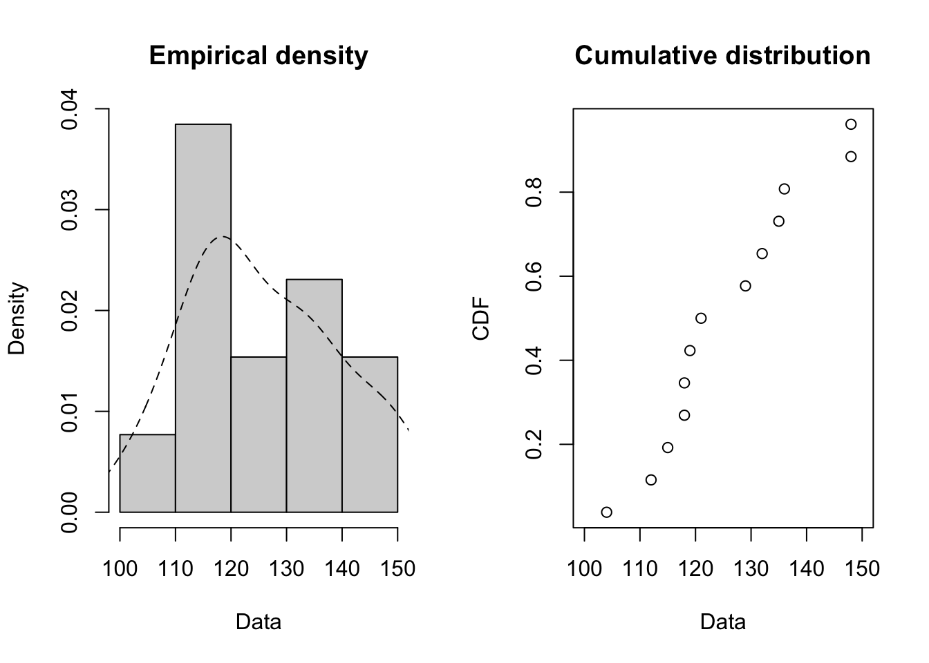
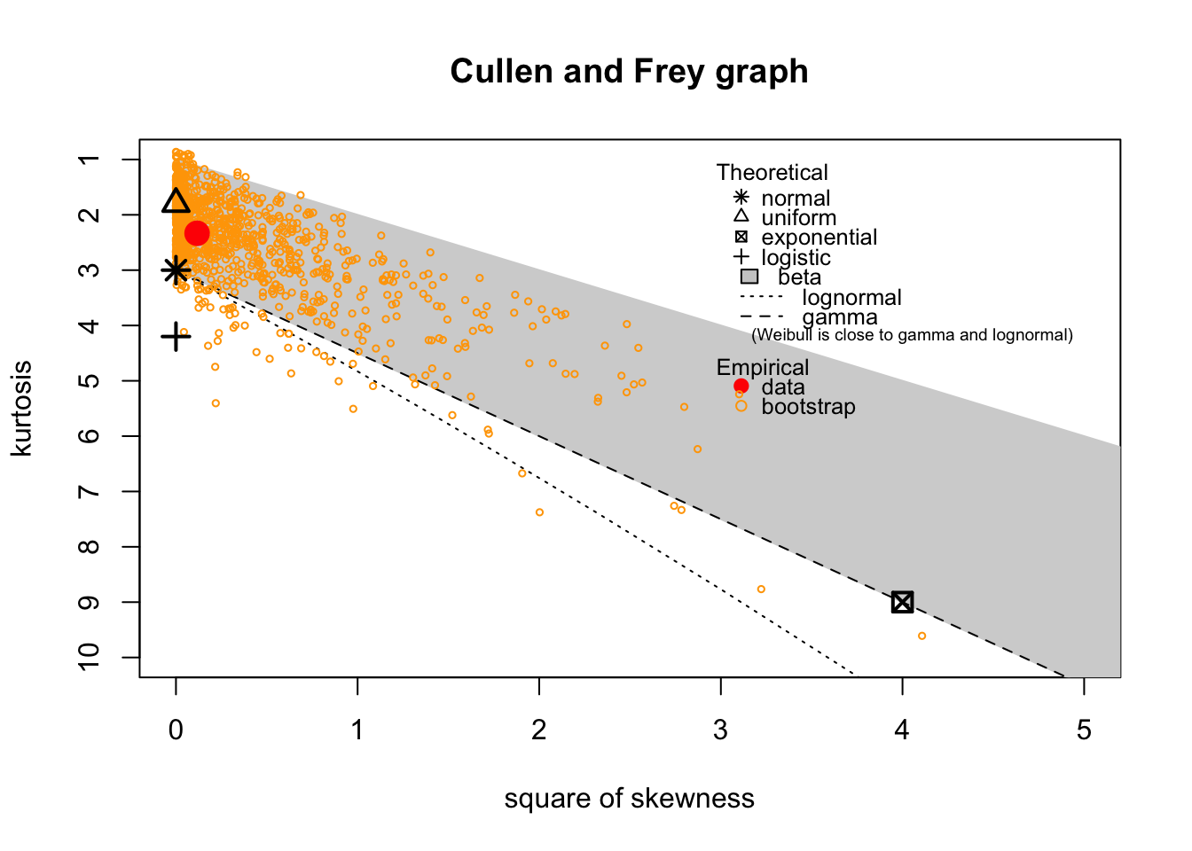
To compute the Skewness–Kurtosis Plot, the R code uses two functions from the fitdistrplus library: plotdist and descdist. The Skewness–Kurtosis Plot is also known as the Cullen and Frey graph (Cullen and Frey 1999).

67.15 Purpose

The Skewness and Kurtosis tests are used to test whether the data are normally distributed or not. The Null Hypothesis states that the Skewness and Kurtosis correspond to a normally distributed variate. If the Null Hypothesis of either Skewness or Kurtosis is rejected, we have to conclude that the data are not normally distributed. Note that the principles of Hypothesis Testing are explained in Hypothesis Testing.

The Skewness–Kurtosis Plot is an explorative tool which allows one to find out whether the data can be described by one of the following distributions:

• The Uniform Distribution.
• The Normal Distribution.
• The Logistic Distribution.
• The Exponential Distribution.
• The Lognormal Distribution (which is represented by a linear equation).
• The Gamma Distribution (which is represented by a linear equation).
• The Beta Distribution (which is shown as a shaded area).
• The Weibull Distribution which is similar to the Gamma and Lognormal line.

67.16 Pros & Cons

67.16.1 Pros of the Skewness & Kurtosis Tests

Skewness and Kurtosis tests have the following advantages:

• They provide an unambiguous answer and are easy to interpret
• They are relatively easy to compute with most statistical software packages

67.16.2 Cons of the Skewness & Kurtosis Tests

Skewness and Kurtosis tests have the following disadvantages:

• They only test for Skewness and Kurtosis, not for other types of centered moments.
• They do not provide information about the type II error (which is what we are really interested in when used as diagnostic tests).
• They are sensitive to outliers.

67.16.3 Pros of the Skewness–Kurtosis Plot

The Skewness-Kurtosis Plot has the following advantages:

• It provides a visual representation of the Kurtosis (y-axis) and squared Skewness (x-axis) of the bootstrap samples of the univariate dataset. Hence, it is easy to determine which distributions could be used to fit the data.
• The bootstrap samples provide an indication of the area of possible Kurtosis \\& Skewness combinations which has an almost similar interpretation as a confidence interval.

67.16.4 Cons of the Skewness–Kurtosis Plot

The Skewness-Kurtosis Plot has the following disadvantages:

• Most readers are not familiar with this plot.
• The Skewness and Kurtosis measure are rather sensitive to outliers.

67.17 Example of Skewness & Kurtosis Tests

We investigate whether or not the birthweight series is normally distributed (based on measures of Kurtosis and Skewness):

Interactive Shiny app (click to load).

Open in new tab

The preliminary conclusion is that the data series is symmetric and that the kurtosis is normal. In Hypothesis Testing we will discuss the interpretation of the hypothesis tests that are shown in the output.

67.18 Example of the Skewness–Kurtosis Plot

The Skewness-Kurtosis Plot for the same data is shown in the following R module:

Interactive Shiny app (click to load).

Open in new tab

The output clearly shows that the area with bootstrap sample points contains the marker of the Normal Distribution. In other words, the Normal Distribution might be used to describe the distribution of the data.

Anscombe, F. J., and William J. Glynn. 1983. “Distribution of the Kurtosis Statistic \(b_2\) for Normal Samples.” Biometrika 70 (1): 227–34. https://doi.org/10.1093/biomet/70.1.227.

Cullen, Alison C., and H. Christopher Frey. 1999. Probabilistic Techniques in Exposure Assessment: A Handbook for Dealing with Variability and Uncertainty in Models and Inputs. New York: Plenum Press.

D’Agostino, Ralph B. 1970. “Transformation to Normality of the Null Distribution of \(g_1\).” Biometrika 57 (3): 679–81. https://doi.org/10.1093/biomet/57.3.679.

D’Agostino, Ralph B., and Michael A. Stephens. 1986. Goodness-of-Fit Techniques. New York: Marcel Dekker.

Geary, R. C. 1935. “The Ratio of the Mean Deviation to the Standard Deviation as a Test of Normality.” Biometrika 27 (3/4): 310–32. https://doi.org/10.2307/2332693.

Jarque, Carlos M., and Anil K. Bera. 1980. “Efficient Tests for Normality, Homoscedasticity and Serial Independence of Regression Residuals.” Economics Letters 6 (3): 255–59. https://doi.org/10.1016/0165-1765(80)90024-5.

Pearson, Karl. 1895. “Contributions to the Mathematical Theory of Evolution. II. Skew Variation in Homogeneous Material.” Philosophical Transactions of the Royal Society of London. Series A 186: 343–414. https://doi.org/10.1098/rsta.1895.0010.

Yule, George Udny. 1911. An Introduction to the Theory of Statistics. London: Charles Griffin; Company.