library(glmnet)

data(mtcars)

x <- model.matrix(mpg ~ . - 1, data = mtcars)
y <- mtcars$mpg

rmse <- function(actual, pred) sqrt(mean((actual - pred)^2))

set.seed(42)
idx <- sample(seq_len(nrow(mtcars)), size = 24)

x_train <- x[idx, ]
x_test <- x[-idx, ]
y_train <- y[idx]
y_test <- y[-idx]161 Regularization Methods
Regularization is used when a regression or classification model is flexible enough to fit the training data too aggressively. The idea is simple: do not let the coefficients move as freely as ordinary fitting would allow.
Instead of minimizing only the residual sum of squares or the negative log-likelihood, a regularized method adds a penalty for large coefficients. The penalty discourages unstable fits and usually improves out-of-sample performance when predictors are numerous, correlated, or both.
This chapter uses glmnet because it provides the three standard penalties in one framework:
| Method | Penalty idea | Practical effect |
|---|---|---|
| Ridge | shrink all coefficients toward zero | keeps every predictor, reduces instability |
| Lasso | shrink coefficients and allow some to become exactly zero | combines shrinkage with variable selection |
| Elastic net | blend ridge and lasso | useful when predictors are both numerous and correlated |
161.1 Why Coefficients Need Shrinkage
When predictors are strongly related to one another, ordinary least squares and ordinary logistic regression can produce coefficients that move around a lot from one sample to the next. The fitted values may still look reasonable, but the individual coefficients become harder to trust.
Regularization does not eliminate the need for good data, sensible predictors, or leakage protection. It does something narrower:
- it reduces coefficient volatility,
- it lowers the chance that the model chases noise,
- it often improves predictive performance on new data.
This is why regularization belongs more naturally to a predictive workflow than to a confirmatory one (see Section 158.2). A lasso model that sets some coefficients to zero can be useful, but it should not be mistaken for a substantive scientific argument about causation.
161.2 The Three Standard Penalties
For linear regression, the ordinary least squares objective is
\[ \sum_{i=1}^{n}(y_i - \hat y_i)^2. \]
Regularization adds a penalty term:
\[ \sum_{i=1}^{n}(y_i - \hat y_i)^2 + \lambda \cdot \text{Penalty}(\beta). \]
The tuning constant \(\lambda\) controls how strongly coefficients are shrunk.
- Ridge regression uses \(\sum_j \beta_j^2\).
- Lasso regression uses \(\sum_j |\beta_j|\).
- Elastic net uses a weighted blend of the two.
The second tuning constant is therefore alpha:
alpha = 0gives ridge,alpha = 1gives lasso,- values between
0and1give elastic net.
The key practical point is that the data do not estimate lambda for you automatically. It must be chosen by validation, which is why this chapter connects directly to Chapter 160 and Chapter 162.
161.3 A Small Regression Example with mtcars
The mtcars dataset is small enough that ordinary fitting can be sensitive to the exact training sample. That makes it a convenient teaching example for shrinkage.
This split does two jobs at once:
- the training set is used to fit the regularized models,
- cross-validation inside the training set is used to choose
lambda, - the outer test set is held back for one final comparison.
That separation matters. If the same rows were used both to choose lambda and to report final performance, the comparison would be optimistic.
161.3.1 Coefficient Paths
The next figure shows what happens when lambda changes from weak shrinkage to strong shrinkage.
ridge_fit <- glmnet(x_train, y_train, alpha = 0)
lasso_fit <- glmnet(x_train, y_train, alpha = 1)

par(mfrow = c(1, 2), mar = c(4, 4, 2, 1))
plot(ridge_fit, xvar = "lambda", label = TRUE)
title("Ridge coefficient paths")

plot(lasso_fit, xvar = "lambda", label = TRUE)
title("Lasso coefficient paths")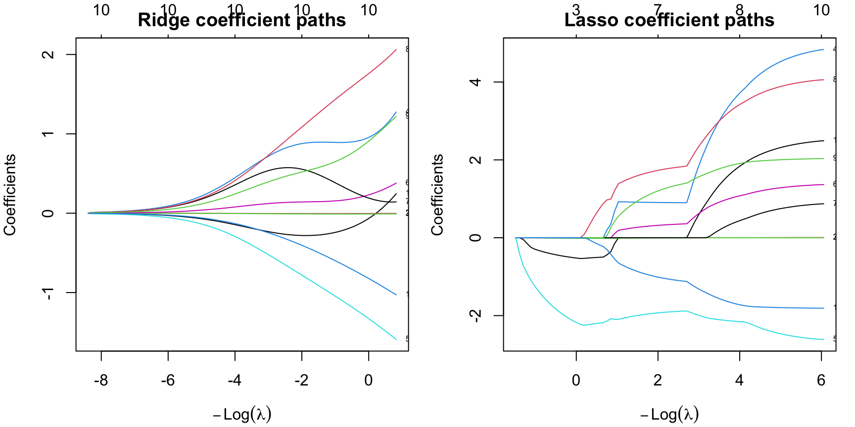
The visual difference is the main lesson:
- ridge shrinks coefficients continuously,
- lasso shrinks them too, but some paths hit exactly zero,
- elastic net sits between those two behaviors.
So the question is not only “Which fit is most accurate?” It is also “How much simplification do we want?”
161.3.2 Choosing lambda by Cross-Validation
cv.glmnet() searches over many lambda values and picks the one that performs best under cross-validation. It also reports a more conservative alternative: the one-standard-error rule.
lambda.minis the value with the lowest cross-validated error,lambda.1seis the largest value whose error is still within one standard error of the minimum.
In practice, lambda.1se often gives a slightly simpler and more stable model.
ridge_cv <- cv.glmnet(x_train, y_train, alpha = 0, nfolds = 5)
lasso_cv <- cv.glmnet(x_train, y_train, alpha = 1, nfolds = 5)
enet_cv <- cv.glmnet(x_train, y_train, alpha = 0.5, nfolds = 5)

summarise_fit <- function(name, cvfit) {
  co <- as.matrix(coef(cvfit, s = "lambda.1se"))
  nz <- sum(abs(co[-1, 1]) > 0)
  pred <- as.numeric(predict(cvfit, newx = x_test, s = "lambda.1se"))
  data.frame(
    Model = name,
    Lambda1SE = cvfit$lambda.1se,
    TestRMSE = rmse(y_test, pred),
    ActiveCoefficients = nz
  )
}

reg_compare <- rbind(
  summarise_fit("Ridge", ridge_cv),
  summarise_fit("Lasso", lasso_cv),
  summarise_fit("Elastic net", enet_cv)
)

knitr::kable(
  transform(
    reg_compare,
    Lambda1SE = round(Lambda1SE, 3),
    TestRMSE = round(TestRMSE, 3)
  ),
  caption = "Outer-test comparison after choosing lambda by inner cross-validation"
)| Model | Lambda1SE | TestRMSE | ActiveCoefficients |
|---|---|---|---|
| Ridge | 10.392 | 4.582 | 10 |
| Lasso | 1.439 | 4.860 | 3 |
| Elastic net | 2.177 | 4.805 | 7 |
In this run:
- ridge gives the lowest outer-test
RMSE, - lasso gives the sparsest model,
- elastic net sits between them on both complexity and error.
That is the regularization tradeoff in one table: accuracy, simplicity, and stability do not always point to the same choice.
161.3.3 What Shrinkage Looks Like Numerically
ridge_coef <- round(as.matrix(coef(ridge_cv, s = "lambda.1se")), 3)
lasso_coef <- round(as.matrix(coef(lasso_cv, s = "lambda.1se")), 3)

coef_compare <- data.frame(
  Predictor = rownames(ridge_coef),
  Ridge = ridge_coef[, 1],
  Lasso = lasso_coef[, 1]
)

knitr::kable(
  coef_compare,
  caption = "Ridge versus lasso coefficients at lambda.1se"
)| Predictor | Ridge | Lasso | |
|---|---|---|---|
| (Intercept) | (Intercept) | 18.680 | 30.261 |
| cyl | cyl | -0.272 | -0.465 |
| disp | disp | -0.004 | 0.000 |
| hp | hp | -0.008 | -0.011 |
| drat | drat | 0.843 | 0.000 |
| wt | wt | -0.691 | -1.945 |
| qsec | qsec | 0.138 | 0.000 |
| vs | vs | 0.574 | 0.000 |
| am | am | 0.964 | 0.000 |
| gear | gear | 0.481 | 0.000 |
| carb | carb | -0.346 | 0.000 |
The ridge model keeps every predictor in the model, but many are small. The lasso model keeps only a few predictors away from zero. That does not mean the dropped variables are scientifically irrelevant. It means the lasso does not need them to optimize this predictive fit at this penalty level.
161.4 The Same Logic in Logistic Regression
Regularization is not limited to linear regression. The same glmnet framework works for binomial outcomes.
library(MASS)
data("Pima.tr", package = "MASS")

x_pima <- model.matrix(type ~ . - 1, data = Pima.tr)
y_pima <- Pima.tr$type

set.seed(123)
lasso_logit <- cv.glmnet(
  x_pima, y_pima,
  family = "binomial",
  alpha = 1,
  nfolds = 5
)

lasso_logit_coef <- round(as.matrix(coef(lasso_logit, s = "lambda.1se")), 3)
lasso_logit_coef <- data.frame(
  Predictor = rownames(lasso_logit_coef),
  Coefficient = lasso_logit_coef[, 1]
)

knitr::kable(
  subset(lasso_logit_coef, Coefficient != 0),
  caption = "Nonzero coefficients from a lasso-logistic fit on Pima.tr"
)| Predictor | Coefficient | |
|---|---|---|
| (Intercept) | (Intercept) | -5.498 |
| npreg | npreg | 0.024 |
| glu | glu | 0.021 |
| bmi | bmi | 0.030 |
| ped | ped | 0.509 |
| age | age | 0.025 |
Here the lasso keeps only a subset of the predictors. The practical reading rule is the same as before:
- this is useful for prediction,
- it can simplify the model,
- but it should not be interpreted as a proof that the dropped variables “do not matter” in the underlying phenomenon.
161.5 Try Regularization in the Apps
The apps now expose regularization in two different styles:
- the app in the menu
Models / Manual Model Buildinglets you turn regularization on explicitly in theGLMandRegressiontabs, - the Guided Model Building app includes regularized logistic and regularized linear regression as candidate models and reports the selected tuning results in the fitted model details.
161.5.1 Manual Model Building: Explicit Search on the GLM Tab
In the manual app, choose GLM, switch Regularization / hyperparameter search away from None, and then click Fit regularized GLM. The app runs the fit asynchronously and shows a wait/progress message if another heavy search is already running.
This view is useful because it makes the tuning decision visible. You can switch between ridge, lasso, elastic net, or an automatic penalty-family search and then inspect which coefficients remain active. The same regularization control also appears in the Regression tab for continuous outcomes.
161.5.2 Guided Model Building: Regularized Candidates Inside a Workflow
The guided app treats regularization differently. Instead of asking the learner to launch a large free-form search, it includes regularized coefficient models directly in the candidate set and tunes the penalty family inside the training rows only.
WarningFull-screen use
The Guided Model Building app is still much easier to read in a new tab, but the embedded panel below loads the regularized Pima session directly if you want to inspect the workflow from inside the chapter first.
In that session, the most important places to look are:
Models, where the regularized logistic fit lists the selected penalty family,alpha,lambda.min,lambda.1se, and the nonzero coefficients,Diagnostics, where you can compare its repeated-validation behavior with the other classifiers,Export, where the R script reconstructs theglmnetpath transparently.
The manual and guided apps therefore teach two complementary regularization habits:
- manual workflow: choose and launch the search yourself,
- guided workflow: compare a tuned shrinkage path against other candidate models inside a controlled validation workflow.
161.6 Practical Reading Rule
Use regularization when the goal is prediction and the coefficient pattern looks too unstable to trust unpenalized fitting.
- Prefer ridge when you want shrinkage but do not want to drop predictors.
- Prefer lasso when you also want automatic sparsity.
- Prefer elastic net when predictors are correlated and pure lasso feels too aggressive.
- Prefer the one-standard-error rule when a slightly simpler model performs essentially as well as the apparent optimum.
161.7 Practical Exercises
- Refit the
mtcarsexample with a different random split. Does the identity of the lowest-RMSEmethod stay the same? - Compare
lambda.minandlambda.1sefor the lasso fit. How many active coefficients do you gain or lose? - Change the elastic-net mixing parameter from
0.5to0.2and then to0.8. How does the coefficient pattern move toward ridge or lasso? - In the
Pima.trlogistic example, compare the nonzero coefficient set atlambda.minandlambda.1se. Which rule gives the simpler classifier?