Logistic regression is a statistical method for modeling the probability of a binary outcome as a function of one or more predictor variables. Unlike linear regression (Chapter 134) which predicts a continuous response, logistic regression predicts the probability that an observation belongs to one of two categories.
The model is widely used in classification problems where the outcome variable \(Y\) takes values 0 or 1 (e.g., disease/no disease, fraud/no fraud, success/failure).
136.2 Why Not Linear Regression?
Consider modeling a binary outcome \(Y \in \{0, 1\}\) using linear regression:
\[
P(Y = 1 | X) = \beta_0 + \beta_1 X
\]
This approach has fundamental problems:
Predicted probabilities can fall outside the valid range \([0, 1]\)
The relationship between \(X\) and the probability is assumed to be linear, which is often unrealistic
The error terms cannot be normally distributed when the outcome is binary
Logistic regression addresses these issues by modeling the probability through a transformation that constrains predictions to lie between 0 and 1.
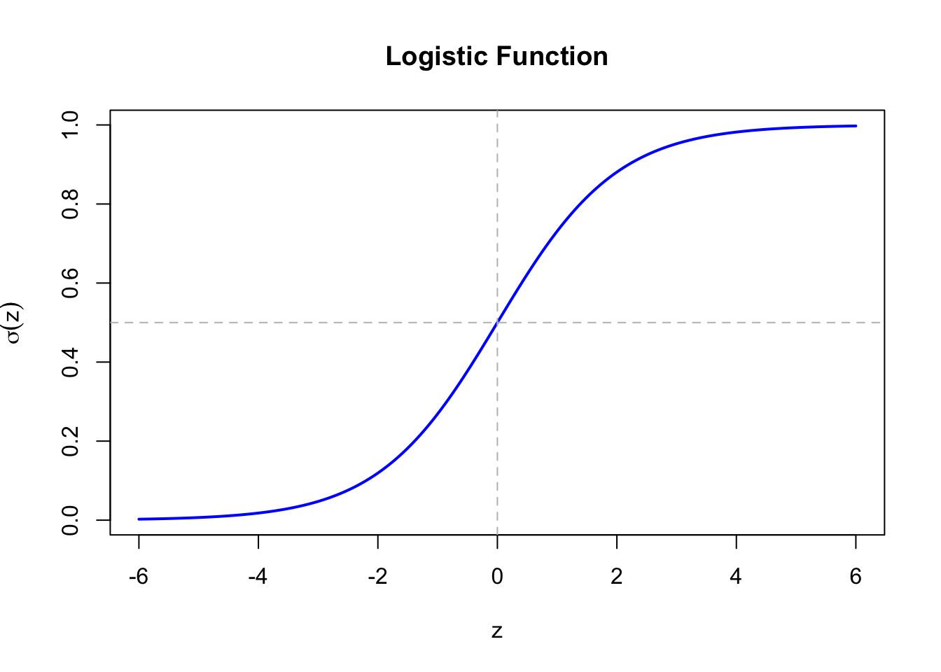
136.3 The Logistic Function
The logistic (sigmoid) function maps any real number to the interval \((0, 1)\):
The quantity \(\frac{p}{1-p}\) is called the odds. If \(p = 0.75\), the odds are \(\frac{0.75}{0.25} = 3\), meaning success is three times more likely than failure.
The logit transforms probabilities from \((0, 1)\) to \((-\infty, +\infty)\), allowing us to use a linear model on this transformed scale.
136.5 Model Specification
The logistic regression model specifies that the log-odds of the outcome is a linear function of the predictors:
The parameters \(\beta_0, \beta_1, ..., \beta_k\) are estimated using maximum likelihood estimation. Given \(n\) independent observations \((x_i, y_i)\) where \(y_i \in \{0, 1\}\), the likelihood function is:
There is no closed-form solution; the estimates are obtained through iterative numerical optimization (typically Newton-Raphson or iteratively reweighted least squares).
136.7 Interpretation of Coefficients
136.7.1 Log-Odds Interpretation
The coefficient \(\beta_j\) represents the change in the log-odds of the outcome for a one-unit increase in \(X_j\), holding other predictors constant.
136.7.2 Odds Ratio Interpretation
Exponentiating the coefficient gives the odds ratio:
\[
\text{OR}_j = e^{\beta_j}
\]
The odds ratio represents the multiplicative change in the odds for a one-unit increase in \(X_j\):
\(\text{OR} > 1\): the predictor increases the odds of \(Y = 1\)
\(\text{OR} = 1\): no effect (equivalent to \(\beta = 0\))
\(\text{OR} < 1\): the predictor decreases the odds of \(Y = 1\)
For example, if \(\beta_1 = 0.693\), then \(\text{OR}_1 = e^{0.693} \approx 2\). A one-unit increase in \(X_1\) doubles the odds of \(Y = 1\).
136.8 Hypothesis Testing
136.8.1 Wald Test
The Wald test evaluates whether a coefficient is significantly different from zero:
\[
z = \frac{\hat{\beta}_j}{\text{SE}(\hat{\beta}_j)}
\]
Under the null hypothesis \(H_0: \beta_j = 0\), the test statistic follows approximately a standard normal distribution for large samples.
Under the null hypothesis, \(G^2\) follows a chi-squared distribution with degrees of freedom equal to the difference in the number of parameters.
136.9 Model Fit and Diagnostics
136.9.1 Deviance
The deviance measures the goodness of fit:
\[
D = -2 \ell(\hat{\beta})
\]
Lower deviance indicates better fit. The null deviance (intercept-only model) can be compared to the residual deviance (full model) to assess the contribution of predictors.
136.9.2 Pseudo R-squared
Unlike linear regression, logistic regression does not have a true \(R^2\). Several pseudo R-squared measures exist:
Values between 0.2 and 0.4 are often considered good fit, but this is only a rough heuristic and depends on context and on which pseudo-\(R^2\) definition is used.
136.9.3 Hosmer-Lemeshow Test
This test (Hosmer and Lemeshow 2000) groups observations into deciles based on predicted probabilities and compares observed and expected frequencies using a chi-squared test.
# Optional: Hosmer-Lemeshow goodness-of-fit test# install.packages("ResourceSelection")library(ResourceSelection)hoslem.test(model$y, fitted(model), g =10)
136.10 Predictions and Classification
Logistic regression produces predicted probabilities \(\hat{p}_i = P(Y = 1 | X = x_i)\). To convert these into binary predictions, a classification threshold must be chosen, as discussed in Section 60.2.
However, the optimal threshold depends on the costs of different types of errors. The ROC curve (Chapter 60) and pay-off matrix (Section 60.5) provide tools for selecting the appropriate threshold.
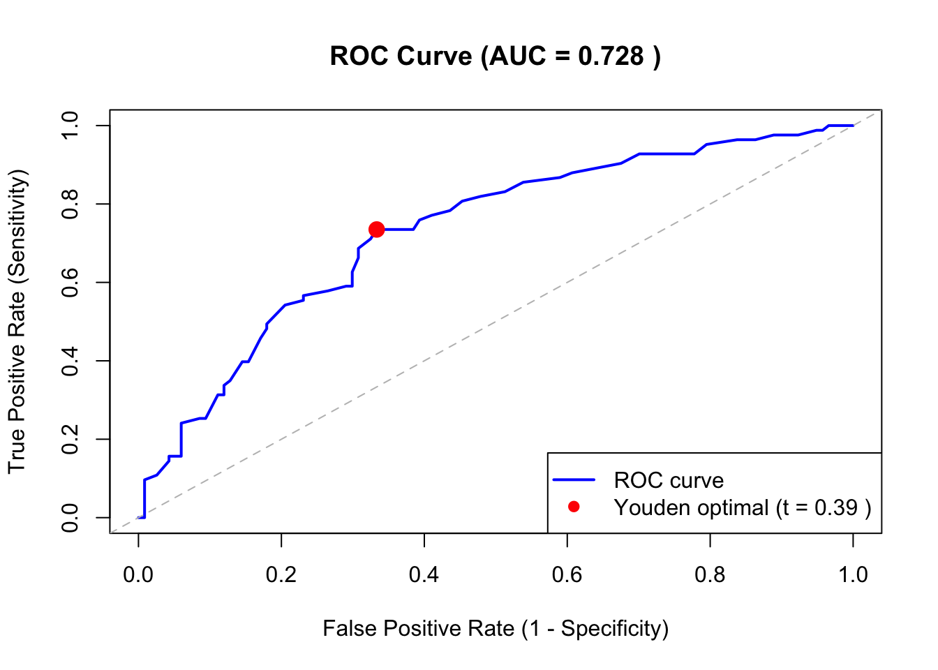
136.11 Connection to ROC Analysis
The predicted probabilities from logistic regression are exactly the type of classifier output that ROC analysis evaluates. The workflow is:
Fit a logistic regression model
Obtain predicted probabilities for all observations
Construct the ROC curve by varying the classification threshold
Compute the AUC to assess overall discriminative ability (Section 60.4)
Select the optimal threshold based on Youden’s index (Youden 1950) or a pay-off matrix (Section 60.5)
The Confusion Matrix (Chapter 59) and associated metrics (Sensitivity, Specificity, Precision) can then be computed at the chosen threshold.
136.12 R Module
136.12.1 Public website
Logistic Regression is available on the public website:
The Logistic Regression module is available in RFC under the menu “Models / Logistic Regression”.
An interactive model-building application that includes logistic regression alongside other classification methods (naive Bayes, conditional inference trees) is available under “Models / Manual Model Building”. This application allows users to compare model performance using ROC curves (Chapter 60) and confusion matrices (Chapter 59), and to select optimal classification thresholds based on cost analysis (Section 60.5).
136.12.3 R Code
The following example demonstrates logistic regression using simulated data:
# Simulate dataset.seed(42)n <-200# Predictorsage <-rnorm(n, mean =50, sd =10)income <-rnorm(n, mean =50000, sd =15000)# True relationship: log-odds depends on age and incomelog_odds <--5+0.05* age +0.00004* incomeprob <-1/ (1+exp(-log_odds))outcome <-rbinom(n, 1, prob)# Create data framedata <-data.frame(outcome, age, income)# Fit logistic regressionmodel <-glm(outcome ~ age + income, data = data, family = binomial)summary(model)
Call:
glm(formula = outcome ~ age + income, family = binomial, data = data)

Coefficients:
              Estimate Std. Error z value Pr(>|z|)
(Intercept) -5.107e+00  1.124e+00  -4.544 5.52e-06 ***
age          3.489e-02  1.663e-02   2.097    0.036 *
income       5.949e-05  1.227e-05   4.848 1.25e-06 ***
---
Signif. codes:  0 '***' 0.001 '**' 0.01 '*' 0.05 '.' 0.1 ' ' 1

(Dispersion parameter for binomial family taken to be 1)

    Null deviance: 271.45  on 199  degrees of freedom
Residual deviance: 240.40  on 197  degrees of freedom
AIC: 246.4

Number of Fisher Scoring iterations: 4
Figure 136.2: ROC Curve for Logistic Regression Model
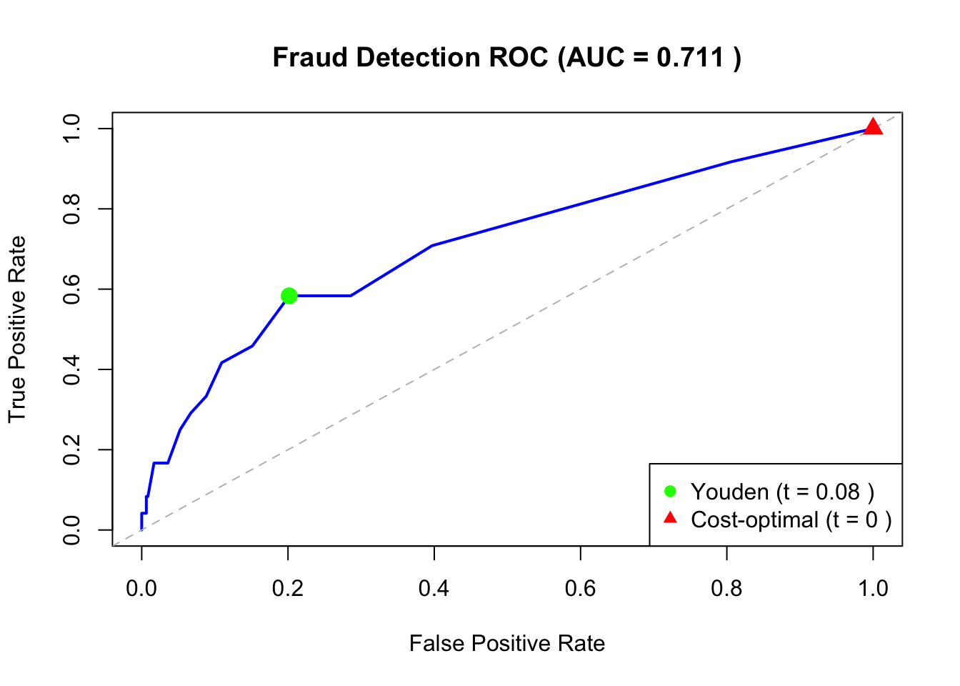
136.13 Example: Fraud Detection
We apply logistic regression to the fraud detection problem introduced in Chapter 58 and Chapter 60.
# Simulated fraud dataset.seed(123)n <-500# Featurestransaction_amount <-rexp(n, rate =0.01) # Transaction amounthour_of_day <-sample(0:23, n, replace =TRUE) # Hour of transactionis_foreign <-rbinom(n, 1, 0.2) # Foreign transaction indicator# True fraud probability depends on featureslog_odds_fraud <--4+0.0005* transaction_amount +0.1* (hour_of_day <6| hour_of_day >22) +1.5* is_foreignprob_fraud <-1/ (1+exp(-log_odds_fraud))is_fraud <-rbinom(n, 1, prob_fraud)fraud_data <-data.frame(is_fraud, transaction_amount, hour_of_day, is_foreign)cat("Fraud rate:", mean(is_fraud), "\n\n")# Fit model# Note: hour_of_day is generated above but excluded here intentionally to keep# the first specification focused on two core predictors.fraud_model <-glm(is_fraud ~ transaction_amount + is_foreign,data = fraud_data, family = binomial)summary(fraud_model)
Fraud rate: 0.048


Call:
glm(formula = is_fraud ~ transaction_amount + is_foreign, family = binomial,
    data = fraud_data)

Coefficients:
                    Estimate Std. Error z value Pr(>|z|)
(Intercept)        -4.012939   0.396641 -10.117  < 2e-16 ***
transaction_amount  0.003877   0.001748   2.218  0.02657 *
is_foreign          1.581474   0.429283   3.684  0.00023 ***
---
Signif. codes:  0 '***' 0.001 '**' 0.01 '*' 0.05 '.' 0.1 ' ' 1

(Dispersion parameter for binomial family taken to be 1)

    Null deviance: 192.58  on 499  degrees of freedom
Residual deviance: 175.26  on 497  degrees of freedom
AIC: 181.26

Number of Fisher Scoring iterations: 6
# Odds ratioscat("\nOdds Ratios:\n")exp(coef(fraud_model))# Interpretation:# - Each $1000 increase in transaction amount multiplies the odds of fraud# - Foreign transactions have much higher odds of being fraudulent
The cost-optimal threshold is lower than Youden’s threshold because missing a fraud (false negative) is much more costly than a false alarm (false positive). This is consistent with the analysis in Chapter 60.
136.14 Separation and Convergence Diagnostics
In practice, logistic regression can fail because of complete or quasi-complete separation (predictors perfectly classify the outcome). Symptoms include very large coefficient estimates, huge standard errors, and convergence warnings.
Recommended workflow:
Check for warnings from glm() (non-convergence, fitted probabilities near 0 or 1).
Inspect sparse cells and near-perfect rules in contingency tables.
If separation is present, use penalized methods (e.g., Firth logistic regression (Firth 1993; Heinze and Schemper 2002)) or simplify the model.
136.15 Multiple Logistic Regression
With multiple predictors, the interpretation extends naturally:
Each coefficient \(\beta_j\) represents the change in log-odds for a one-unit increase in \(X_j\), holding all other predictors constant. This is analogous to the interpretation in multiple linear regression (Chapter 135).
Interaction terms and polynomial terms can be included:
# Interaction between amount and foreign transactionmodel_interaction <-glm(is_fraud ~ transaction_amount * is_foreign,data = fraud_data, family = binomial)# Polynomial term for non-linear effectmodel_poly <-glm(is_fraud ~poly(transaction_amount, 2) + is_foreign,data = fraud_data, family = binomial)
136.16 Assumptions
Logistic regression makes the following assumptions:
Binary outcome: The dependent variable must be binary (or binomial counts)
Independence: Observations are independent of each other
Linearity in log-odds: The relationship between predictors and log-odds is linear
No perfect multicollinearity (identification): Predictors cannot be exact linear combinations of each other
Large sample size: Maximum likelihood estimation requires adequate sample size (rule of thumb: at least 10 events per predictor)
High (imperfect) multicollinearity is a practical estimation concern because it inflates standard errors and can destabilize coefficient estimates.
Unlike linear regression, logistic regression does not assume:
Normality of residuals
Homoscedasticity (constant variance)
Linear relationship between predictors and the outcome
136.17 Pros & Cons
136.17.1 Pros
Logistic regression has the following advantages:
Produces interpretable coefficients as odds ratios.
Outputs probabilities that can be used with ROC analysis for threshold optimization.
Does not require normally distributed predictors.
Handles both continuous and categorical predictors.
Computationally efficient even for large datasets.
136.17.2 Cons
Logistic regression has the following disadvantages:
Assumes a linear relationship between predictors and log-odds, which may not hold.
Sensitive to outliers in the predictor variables.
Requires a relatively large sample size, especially when the outcome is rare.
Cannot directly handle missing data.
May underperform compared to more flexible methods (e.g., random forests, neural networks) when relationships are highly non-linear.
136.18 Task
Using the fraud detection data or a dataset of your choice, fit a logistic regression model. Interpret the coefficients as odds ratios.
Construct the ROC curve for your fitted model and compute the AUC. How does the model’s discriminative ability compare to the AUC interpretation guidelines in Table 60.2?
Define a pay-off matrix appropriate for your application. What is the cost-optimal threshold, and how does it differ from the default threshold of 0.5?
Compare the predictions from logistic regression at the cost-optimal threshold with predictions at the Youden-optimal threshold. Compute the Confusion Matrix (Chapter 59) for both and discuss the trade-offs.
Firth, David. 1993. “Bias Reduction of Maximum Likelihood Estimates.”Biometrika 80 (1): 27–38.
Heinze, Georg, and Michael Schemper. 2002. “A Solution to the Problem of Separation in Logistic Regression.”Statistics in Medicine 21 (16): 2409–19.
Hosmer, David W., and Stanley Lemeshow. 2000. Applied Logistic Regression. 2nd ed. New York: John Wiley & Sons.
McFadden, Daniel. 1974. “Conditional Logit Analysis of Qualitative Choice Behavior.” In Frontiers in Econometrics, edited by Paul Zarembka, 105–42. New York: Academic Press.