Before diving into formulas and methods, let’s step back and ask a simple question: Why do we analyze data in the first place?
The answer to this question determines everything that follows — which methods to use, how to interpret results, and what conclusions we can draw. This chapter provides a roadmap of the entire book by exploring the different reasons people analyze data.
4.1 Four Purposes of Statistical Analysis
When someone collects data and wants to analyze it, they typically have one of four goals in mind:
Describe: Summarize what the data looks like
Explore: Discover patterns, problems, or interesting questions
Infer: Test claims or draw conclusions about a larger population
Predict: Forecast future observations or outcomes
These purposes are not mutually exclusive — a complete analysis often involves all four. But understanding which purpose drives your analysis helps you choose the right tools.
4.1.1 Purpose 1: Description
“What does my data look like?”
Sometimes we simply want to summarize a dataset. A company might want to know the average salary of its employees. A teacher might want to know the typical exam score in their class. A researcher might want to characterize the patients in a clinical trial.
Example: Summarizing Customer Ages
A retail store collects data on 500 customers and wants to describe their age distribution:
# Simulated customer agesset.seed(42)ages <-c(rnorm(300, mean =35, sd =10), rnorm(200, mean =55, sd =8))ages <-pmax(18, pmin(ages, 80)) # Constrain to realistic range# Descriptive summarycat("Number of customers:", length(ages), "\n")
The goal here is purely descriptive — we are summarizing this specific dataset, not making claims about customers in general or predicting future customer ages.
Descriptive methods covered in this book include measures of central tendency (mean, median, mode), variability (variance, standard deviation), and visualization techniques like histograms (Chapter 62) and box plots (Chapter 69).
4.1.2 Purpose 2: Exploration
“What interesting patterns or problems are hiding in my data?”
Exploratory Data Analysis (EDA) goes beyond description. The goal is to discover things we didn’t know to look for: unexpected patterns, outliers, data quality issues, or new research questions.
Example: Discovering a Bimodal Distribution
Looking at the same customer age data, a simple histogram reveals something interesting:
Code
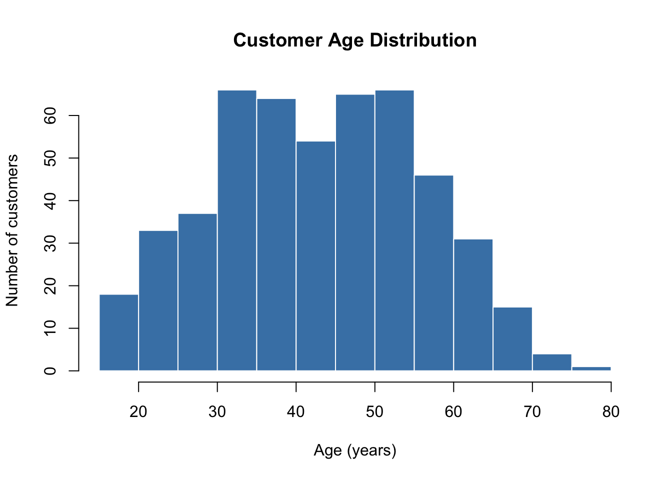
hist(ages, breaks =20, col ="steelblue", border ="white",main ="Customer Age Distribution",xlab ="Age (years)", ylab ="Number of customers")
Figure 4.1: Exploratory histogram reveals two distinct customer groups
The histogram reveals two peaks — the store seems to have two distinct customer groups (younger adults around 35 and older adults around 55). This was not obvious from the summary statistics alone.
This discovery might lead to new questions: Are these groups buying different products? Should marketing strategies differ for each group?
EDA is about asking questions, not answering them. It’s detective work. Tools for exploration include scatter plots, correlation analysis, box plots for comparing groups (Chapter 69), and various diagnostic plots.
4.1.3 Purpose 3: Inference
“Can I draw conclusions about a population based on my sample?”
Inference is about going beyond the data in hand. We use a sample to make claims about a larger population, and we quantify our uncertainty about those claims.
Example: Testing a Claim About Customer Satisfaction
A company claims that at least 80% of customers are satisfied with their service. A consumer organization surveys 200 randomly selected customers and finds that 148 (74%) report being satisfied. Is the company’s claim credible?
# Test the claimsatisfied <-148total <-200claimed_rate <-0.80# One-sample proportion testresult <-prop.test(satisfied, total, p = claimed_rate, alternative ="less")cat("Observed satisfaction rate:", satisfied/total *100, "%\n")
Observed satisfaction rate: 74 %
cat("Claimed rate:", claimed_rate *100, "%\n")
Claimed rate: 80 %
cat("p-value:", round(result$p.value, 4), "\n")
p-value: 0.021
The p-value tells us how likely we would observe 74% satisfaction (or less) if the true rate really were 80%. A small p-value suggests the company’s claim may not be accurate.
This is inference — we’re using sample data to evaluate a claim about all customers, not just the 200 we surveyed.
Inferential methods include hypothesis tests, confidence intervals, and the various tests covered in the Hypothesis Testing part of this book.
4.1.4 Purpose 4: Prediction
“What will happen next?”
Sometimes we want to forecast future observations or predict outcomes for new cases. The focus shifts from understanding why something happens to predicting what will happen.
Example: Predicting House Prices
A real estate company wants to predict house prices based on features like size, location, and age. They have data on 500 past sales and want to predict prices for new listings.
# Simulated house price dataset.seed(123)n <-500size <-runif(n, 800, 3000) # Square feetage <-sample(0:50, n, replace =TRUE) # Yearsprice <-50000+100* size -500* age +rnorm(n, 0, 30000)houses <-data.frame(size, age, price)# Fit a prediction modelmodel <-lm(price ~ size + age, data = houses)# Predict price for a new house: 1800 sq ft, 10 years oldnew_house <-data.frame(size =1800, age =10)predicted_price <-predict(model, new_house)cat("Predicted price for 1800 sq ft, 10-year-old house: $",format(round(predicted_price), big.mark =","), "\n", sep ="")
Predicted price for 1800 sq ft, 10-year-old house: $223,513
Here we don’t care as much about why size and age affect price — we just want accurate predictions for new houses.
The purpose of your analysis determines what you do with the data. Consider this example:
Scenario: A hospital collects data on 1,000 patients, including their age, weight, blood pressure, and whether they developed heart disease.
Table 4.1: Different purposes lead to different analyses
Purpose
Question
Approach
Describe
What is the average blood pressure in our patient population?
Calculate mean, median, standard deviation
Explore
Are there unusual patterns or subgroups in the data?
Create scatter plots, look for clusters, check for outliers
Infer
Is high blood pressure associated with heart disease?
Conduct a hypothesis test comparing blood pressure between groups
Predict
Which patients are likely to develop heart disease?
Build a classification model using logistic regression or decision trees
4.3 Why Purpose Matters: Two Critical Distinctions
4.3.1 Inference vs. Prediction in Modeling
When building a regression model, your purpose fundamentally changes how you evaluate success:
Inference focus (answering scientific questions):
You care about the coefficients: “Does smoking increase disease risk?”
You want p-values and confidence intervals
Interpretability is essential
A simpler model may be better even if it predicts slightly worse
Prediction focus (forecasting new cases):
You care about accuracy on new data
You evaluate using out-of-sample metrics (test set performance)
A complex model is fine if it predicts well
The coefficients themselves may be uninterpretable
Example: A pharmaceutical company studies whether a new drug reduces blood pressure.
For inference: They need to estimate the drug effect (coefficient) with a confidence interval and test whether it’s statistically significant. The model must be interpretable.
For prediction: If they just want to predict a patient’s blood pressure after treatment, they could use any model that predicts well — even a “black box” model.
4.3.2 Description vs. Exploration vs. Residual Analysis
Not all “looking at data” is the same:
Description: Summarizing what you observe
“The average customer spends €47 per visit”
Purpose: Reporting, characterization
Exploration: Discovering the unexpected
“There seem to be two distinct customer groups — I didn’t expect that”
Purpose: Generating hypotheses, finding patterns
Residual analysis: Checking model assumptions
“The residuals from my regression model show a curved pattern — the linear model may not be appropriate”
Purpose: Validating models, diagnosing problems
All three use similar tools (plots, summary statistics) but for different reasons. A histogram during exploration helps you discover patterns. The same histogram of residuals checks whether your model assumptions hold.
4.4 The Role of Probability
Before we can do inference, we need to understand probability and probability distributions. If you flip a coin 100 times and get 60 heads, is the coin biased? To answer this, you need to know what to expect from a fair coin — and that requires understanding the binomial distribution.
The probability chapters (Chapter 5 through the F Distribution) provide the foundation for all inferential methods. They answer questions like:
How much variation should we expect by chance?
What does a “typical” sample look like?
How do we quantify unusual observations?
4.5 Time Series: A Special Case
When data are collected over time, the observations are usually not independent — today’s value depends on yesterday’s. This requires specialized methods:
Time series plots to visualize temporal patterns
Decomposition (Chapter 146) to separate trend, seasonality, and noise
Time series analysis combines all four purposes: describing the series, exploring for patterns, testing for trends or seasonality, and predicting future values.
4.6 Navigating This Book
The book is organized to match these purposes:
Table 4.2: Book organization by purpose
Part
Purpose
Key Question
Introduction to Probability
Foundation
What should we expect by chance?
Probability Distributions
Foundation
What patterns does randomness follow?
Descriptive Statistics & EDA
Describe & Explore
What does the data look like?
Hypothesis Testing
Infer
Can we generalize from sample to population?
Regression Models
Infer & Predict
How are variables related? What will happen?
Time Series Analysis
All four
How do patterns unfold over time?
4.7 Before You Choose a Method
When you have data and want to analyze it, ask yourself:
What is my goal? Am I describing, exploring, testing a hypothesis, or predicting?
What am I assuming? Every method makes assumptions. Am I willing to accept them?
What would convince me? Before looking at results, decide what would change your mind.
Who is my audience? A scientific paper requires different evidence than a business report.
The detailed selection guide in Appendix A provides systematic help for choosing specific methods. But first, be clear about your purpose — the “how” follows from the “why.”
4.8 Summary
Statistical analysis serves four main purposes: description, exploration, inference, and prediction
The same data can be analyzed differently depending on your goal
Inference and prediction require different evaluation criteria
Description, exploration, and residual analysis use similar tools for different reasons
Understanding probability provides the foundation for inference
Time series data require specialized methods due to temporal dependence
The rest of this book provides the tools for each purpose. But always start with the question: Why am I analyzing this data?