Bayesian inference is often a more natural decision framework than mechanical one-alpha testing because it reports probabilities directly in decision terms:
posterior probability of the claim,
posterior probability of being wrong if we act now,
In many applied settings, decision makers do not ask:
“Is the p-value below 5%?”
They ask:
“Given the data, how likely is the claim?”
“How much risk of being wrong remains if we act now?”
“What decision threshold is appropriate for this business context?”
Bayesian inference answers these directly through posterior probabilities.
113.2 Beta-Binomial Update (Core Model)
Suppose an unknown event probability is denoted by \(p\) (for example: fraud rate, conversion rate, default rate).
We observe \(n\) trials and count how many of them are events.
The notation is:
Symbol
Meaning
\(p\)
the unknown underlying event probability in the population or process
\(n\)
the number of observed trials
\(Y\)
the random variable for the number of events in those \(n\) trials before the data are observed
\(y\)
the realized observed number of events after the data are collected
So \(y / n\) is the observed sample proportion, not the true probability itself. It is a data-based estimate of \(p\), but it is not equal to \(p\).
For Binomial data with \(y\) observed events in \(n\) trials:
\[
Y \mid p \sim \text{Binomial}(n, p)
\]
and with a Beta prior:
\[
p \sim \text{Beta}(\alpha_0, \beta_0),
\]
the posterior is:
\[
p \mid y \sim \text{Beta}(\alpha_0 + y,\; \beta_0 + n - y).
\]
A prior is called conjugate for a likelihood when the posterior stays in the same distribution family after updating with data.
In this chapter:
prior: \(p \sim \text{Beta}(\alpha_0,\beta_0)\)
likelihood: \(Y\mid p \sim \text{Binomial}(n,p)\)
posterior: \(p\mid y \sim \text{Beta}(\alpha_0+y,\beta_0+n-y)\)
This matters because updating becomes transparent, fast, and easy to explain in teaching and practice.
113.2.2 Choosing a Beta prior in practice
The Beta prior is not just a technical convenience. It is also easy to interpret:
\[
E(p) = \frac{\alpha_0}{\alpha_0 + \beta_0}.
\]
So:
the ratio \(\alpha_0 / (\alpha_0 + \beta_0)\) sets your best prior guess for the event rate,
the total \(\alpha_0 + \beta_0\) controls how strongly that prior pulls on the posterior.
In practice, you can think of \(\alpha_0 + \beta_0\) as the prior strength in pseudo-observations. A prior such as \(\text{Beta}(3,97)\) says: “before seeing the new data, I expect about 3% events, and I hold that view with roughly the weight of 100 prior observations.”
This is exactly why \(\text{Beta}(3,97)\), \(\text{Beta}(30,970)\), and \(\text{Beta}(300,9700)\) are not equivalent even though they all have prior mean \(0.03\):
\(\text{Beta}(3,97)\) has prior strength \(100\),
\(\text{Beta}(30,970)\) has prior strength \(1000\),
\(\text{Beta}(300,9700)\) has prior strength \(10000\).
All three priors say “I expect about 3% events,” but they differ in how stubborn that belief is. A stronger prior is harder for the new data to move. It is therefore useful to separate two ideas:
the mean tells you where the prior is centered,
the strength tells you how strongly it resists being updated.
113.3 Decision Rule in Posterior Terms
Define a business-relevant claim, for example \(p < p_0\) or \(p > p_0\).
Here \(p_0\) is the decision threshold that separates acceptable from unacceptable values of the event probability. For example, if management says “the fraud rate must be below 2%,” then \(p_0 = 0.02\).
Then compute the posterior probability of that claim:
\[
q = P(\text{claim} \mid \text{data}).
\]
Choose a decision threshold \(\tau\) by context (confirmatory, balanced, diagnostic):
\[
\text{Support claim if } q \ge \tau.
\]
This makes the threshold explicit and interpretable:
For point-null comparison, we can compare two competing statistical statements:
\(H_0\): the event probability is fixed exactly at the threshold value, \(p = p_0\),
\(H_1\): the event probability is not fixed at one value; instead, many plausible values of \(p\) are allowed, weighted by a Beta prior.
So when this chapter says “\(H_1\) with a Beta prior,” it means that under \(H_1\) we do not commit to one single value of \(p\). We spread prior belief across a whole range of possible values of \(p\) using a Beta distribution.
It quantifies relative evidence between models, while \(P(p < p_0 \mid \text{data})\) answers a directional posterior claim about the parameter.
These are related but distinct: \(\text{BF}_{10}\) compares \(H_0: p=p_0\) to the full \(H_1\) prior (all plausible \(p\) values), so \(\text{BF}_{10}\) and \(P(p < p_0 \mid \text{data})\) can point in different directions.
113.4.2 How large should BF10 be?
Students often ask for a single universal cutoff (for example: BF10 > 3 or > 10).
This is usually the wrong first question for the same reason that one fixed alpha is problematic.
A better workflow is:
specify the decision context and the costs of errors,
report the Bayes factor and posterior model probability,
show sensitivity to alternative reasonable priors,
then decide whether evidence is sufficient for the concrete decision.
So Bayes-factor thresholds are context guides, not universal constants.
For orientation, however, students often benefit from a first reading scale:
\(\text{BF}_{10}\)
Rough classroom interpretation
about 1
little separation between \(H_1\) and \(H_0\)
3 to 10
moderate support for \(H_1\)
greater than 10
strong support for \(H_1\)
below 1
evidence tilts toward \(H_0\) instead
This table is only a starting point. It should never replace context, prior sensitivity, and a clear statement of the actual decision threshold.
113.4.3 Bayes Error Rate (Theoretical vs Operational)
In binary decision settings, two different quantities are often called “Bayes error”:
Theoretical Bayes error rate: minimum achievable misclassification probability under the true class-conditional distributions (not directly computable in practical finite-data settings).
Operational posterior decision error: threshold-dependent local decision error computed from posterior class probabilities.
The reason both appear in the literature is that they answer different questions:
the theoretical quantity is a benchmark or lower bound,
the operational quantity is what you can actually compute from model-based posterior scores in practice.
For the operational quantity, once posterior class probabilities are available, each case has a local decision error probability:
if classify as positive: \(1 - P(\text{positive}\mid x)\),
if classify as negative: \(P(\text{positive}\mid x)\).
The average of these local error probabilities over evaluated cases provides a practical, threshold-dependent decision error summary.
The R snippet below reports this operational quantity.
113.5 Business Example: Fraud-Rate Decision
Assume a payment team deploys a new rule and wants to support the operational claim:
\[
p < 0.02
\]
where \(p\) is the underlying fraud rate after deployment.
Prior belief from historical process knowledge:
\[
p \sim \text{Beta}(3, 97)
\]
(prior mean \(= \alpha_0 / (\alpha_0 + \beta_0) = 3 / 100 = 3\%\)).
Observed in a recent batch: \(y=7\) fraud events out of \(n=400\).
The observed fraud rate in the batch is
\[
\hat{p} = \frac{7}{400} = 0.0175,
\]
which is below the target threshold of 2%. Even so, the posterior probability of the claim will not automatically be high, because the prior mean was 3% and 400 observations do not completely overwhelm that prior.
113.5.1 R snippet 1: posterior update and decision summary
# Prior and dataalpha0 <-3beta0 <-97n <-400y <-7p0 <-0.02tau <-0.90# decision threshold for P(p < p0 | data)# Posterioralpha_post <- alpha0 + ybeta_post <- beta0 + n - yprior_mean <- alpha0 / (alpha0 + beta0)observed_rate <- y / npost_mean <- alpha_post / (alpha_post + beta_post)post_prob_claim <-pbeta(p0, shape1 = alpha_post, shape2 = beta_post) # P(p < p0 | data)ci90 <-qbeta(c(0.05, 0.95), shape1 = alpha_post, shape2 = beta_post)decision <-if (post_prob_claim >= tau) "Support claim p < 0.02"else"Do not support claim yet"if (post_prob_claim >= tau) { risk_label <-"Probability of decision error if we support the claim now" risk_value <-1- post_prob_claim} else { risk_label <-"Probability the claim is true even though we do not support it yet" risk_value <- post_prob_claim}summary_tab <-data.frame(quantity =c("Prior mean","Observed rate","Posterior mean","P(p < 0.02 | data)","90% credible interval","Decision", risk_label ),value =c(sprintf("%.4f", prior_mean),sprintf("%.4f", observed_rate),sprintf("%.4f", post_mean),sprintf("%.4f", post_prob_claim),sprintf("[%.4f, %.4f]", ci90[1], ci90[2]), decision,sprintf("%.4f", risk_value) ))knitr::kable(summary_tab, col.names =c("Summary", "Value"))
Summary
Value
Prior mean
0.0300
Observed rate
0.0175
Posterior mean
0.0200
P(p < 0.02 | data)
0.5408
90% credible interval
[0.0109, 0.0313]
Decision
Do not support claim yet
Probability the claim is true even though we do not support it yet
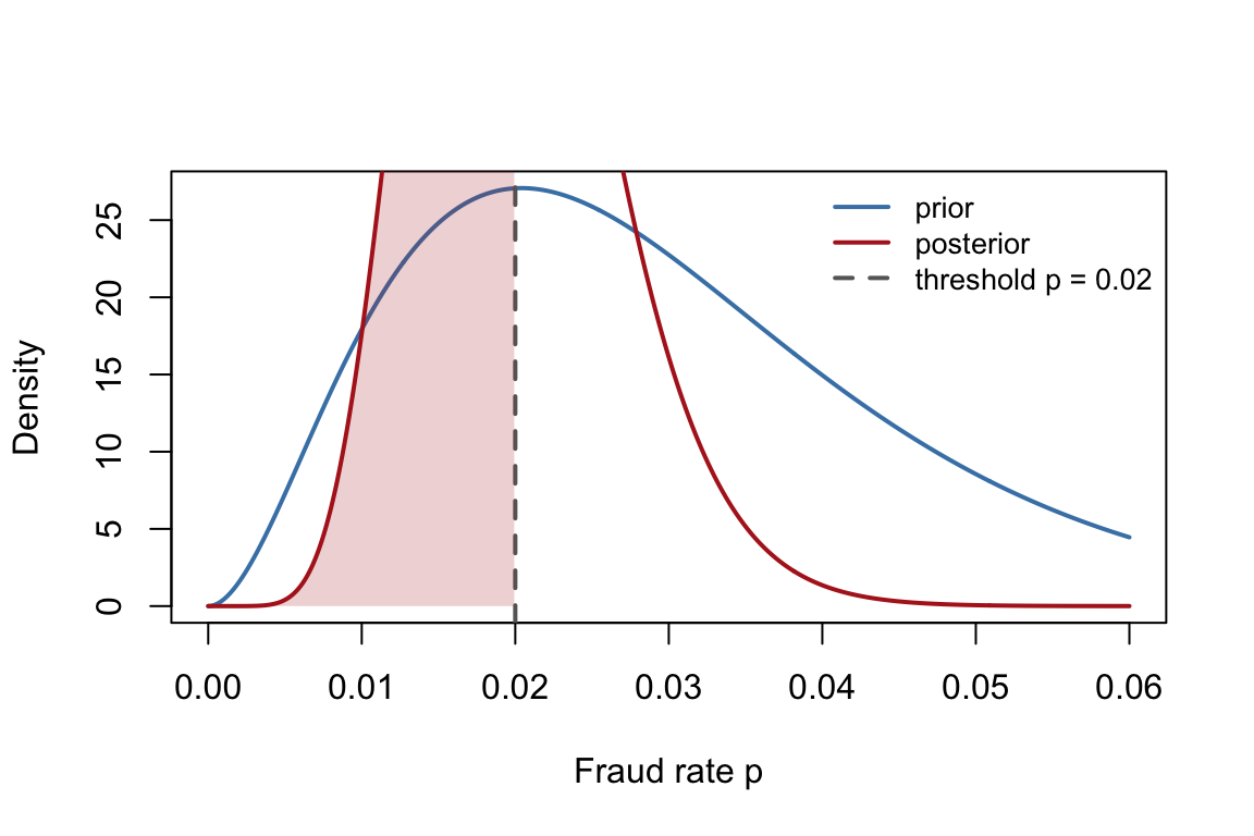
Prior and posterior Beta densities for the fraud-rate example. The vertical line marks the operational claim threshold p = 0.02.
The shaded posterior area to the left of \(p_0 = 0.02\) is exactly the probability used in the decision rule:
\[
P(p < 0.02 \mid \text{data}) \approx 0.54.
\]
That makes the decision logic easier to interpret: even though the observed rate is below 2%, the posterior mass below 2% is still only about 54%, far below the decision threshold \(\tau = 0.90\).
113.5.3 R snippet 3: sensitivity to alternative reasonable priors
This table is not an argument for changing priors until a desired decision appears. It is a reminder that Bayesian decisions should be accompanied by reasonable prior sensitivity checks.
113.5.4 R snippet 4: Bayes factor for a point-null comparison
# Bayes factor H0: p = p0 versus H1: p ~ Beta(alpha0, beta0)log_m1 <-lchoose(n, y) +lbeta(alpha_post, beta_post) -lbeta(alpha0, beta0)log_m0 <-lchoose(n, y) + y *log(p0) + (n - y) *log(1- p0)bf10 <-exp(log_m1 - log_m0)cat("BF10 (H1 vs H0: p = 0.02) =", round(bf10, 6), "\n")
BF10 (H1 vs H0: p = 0.02) = 0.428271
Here the Bayes factor is slightly below 1, so it tilts mildly toward the point null \(H_0: p = 0.02\). That does not contradict the posterior claim probability above. The two quantities answer different questions:
the posterior claim probability asks whether \(p\) is below 0.02,
the Bayes factor compares one exact point null against the whole alternative prior.
113.5.5 R snippet 5: practical Bayes decision error on scored cases
# The fraud-rate example above concerned one population parameter p.# In a scoring system, we instead work with posterior probabilities for individual cases.# The values below are illustrative case-level scores; they are not computed from the Beta-Binomial example above.post_fraud <-c(0.03, 0.08, 0.12, 0.19, 0.27, 0.44, 0.61, 0.74, 0.86, 0.93)threshold <-0.25pred_label <-ifelse(post_fraud >= threshold, "fraud", "legit")local_error <-ifelse(pred_label =="fraud", 1- post_fraud, post_fraud)cat("Average local decision error probability =", round(mean(local_error), 5), "\n")
For threshold selection across contexts: Chapter 112
For posterior analysis in two-sample settings: Chapter 122
113.7 Practical Takeaway
Bayesian inference does not remove the need for threshold choice. It improves the workflow by making thresholds explicit in posterior probability terms and by reporting decision risk directly.
113.8 Practical Exercises
Recompute the fraud example with \(\text{Beta}(1,1)\) instead of \(\text{Beta}(3,97)\). How much does \(P(p < 0.02 \mid \text{data})\) change?
Keep the prior \(\text{Beta}(3,97)\) but change the batch to \(y = 20\) frauds out of \(n = 1000\). Does the claim \(p < 0.02\) now reach a 90% decision threshold?
In the scored-case example, raise the threshold from 0.25 to 0.60. What happens to the average local decision error?
Explain in your own words why \(\text{BF}_{10}\) and \(P(p < p_0 \mid \text{data})\) are not the same quantity, even when they are based on the same observed data.