102 The Central Limit Theorem (revisited)

The Central Limit Theorem is one the most important theorems in inferential statistics. Henceforth, we use a different notation which is more conventional. Information about samples is now represented by small symbols (such as \(n\) for the sample size and \(\bar{x}\) for the Arithmetic Sample Mean). In addition, we use the following notation to indicate that a (population) variable \(X\) is normally distributed with \(E(X) = \mu\) and \(V(X) = \sigma^2\):

\[X \sim \text{N}\left(\mu, \sigma^2\right)\]

Unless stated otherwise, all samples are assumed to be simple random samples.

Central Limit Theorem

If there exists a population with a random variable \(X \sim \text{G} \left( \mu, \sigma^2 \right)\), where \(G\) is an arbitrary distribution with finite variance, then the arithmetic sample mean \(\bar{X}\), obtained from independently and randomly drawn sample observations, is approximately normally distributed with mean \(\mu\) and variance \(\frac { \sigma^2 } { n }\) provided that \(n\) is sufficiently large.

Note that the sampling distribution has a variance \(\frac { \sigma^2 } { n }\) that is smaller than the original variance \(\sigma^2\).

102.1 How large should \(n\) be?

There is no universal threshold. The required sample size depends on the shape of the population distribution:

Mildly skewed distributions: normal approximation is often reasonable around \(n \approx 30\).
Strongly skewed or heavy-tailed distributions: larger samples (often \(n \geq 100\)) may be needed.
If variance does not exist (e.g. Cauchy distribution), the usual CLT does not apply.

So “large enough” is a modeling judgment, not a fixed rule.

102.2 Worked Example

Assume a population with mean \(\mu = 50\) and standard deviation \(\sigma = 12\).
For samples of size \(n = 36\), the CLT gives

\[\bar{X} \approx N\!\left(50,\frac{12^2}{36}\right)=N(50,4)\]

so the standard error is

\[SE(\bar{X}) = \frac{\sigma}{\sqrt{n}} = \frac{12}{6} = 2\]

Hence, as a quick approximation,

\[P(48 \le \bar{X} \le 52) \approx P(-1 \le Z \le 1) \approx 0.6827\]

This is exactly the type of approximation used throughout hypothesis testing and confidence intervals.

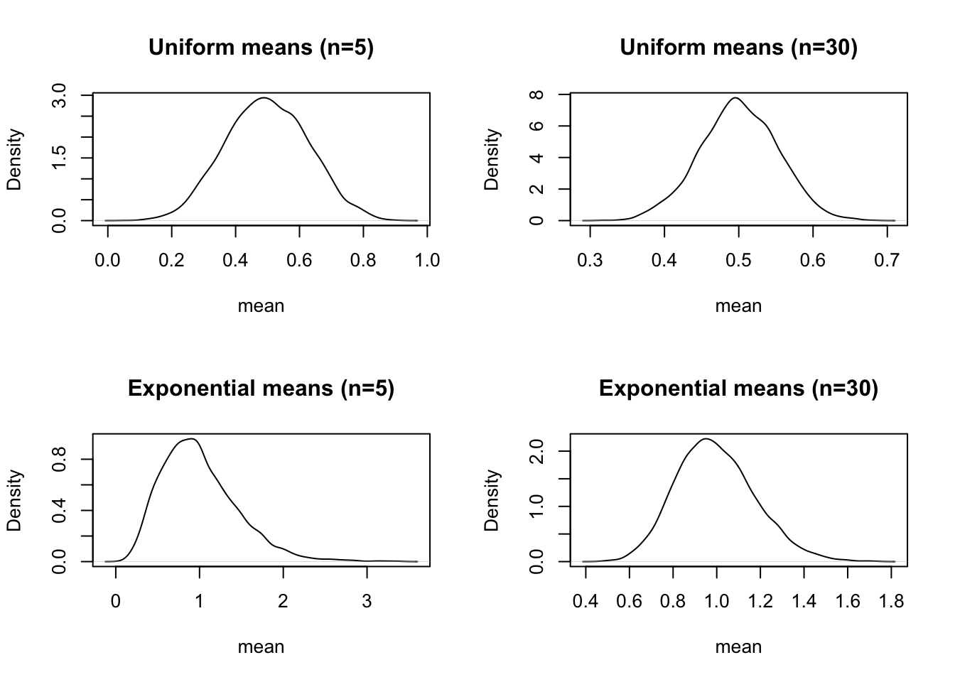
102.3 Simulation Illustration

The following code compares sampling distributions of the mean for two non-normal populations (uniform and exponential), at small and larger sample sizes.

set.seed(123)
B <- 5000

# Uniform(0,1): symmetric, finite variance
m_u_5  <- replicate(B, mean(runif(5, min = 0, max = 1)))
m_u_30 <- replicate(B, mean(runif(30, min = 0, max = 1)))

# Exponential(rate=1): skewed, finite variance
m_e_5  <- replicate(B, mean(rexp(5, rate = 1)))
m_e_30 <- replicate(B, mean(rexp(30, rate = 1)))

# Defensive cleanup for plotting
m_u_5  <- m_u_5[is.finite(m_u_5)]
m_u_30 <- m_u_30[is.finite(m_u_30)]
m_e_5  <- m_e_5[is.finite(m_e_5)]
m_e_30 <- m_e_30[is.finite(m_e_30)]

par(mfrow = c(2,2))
plot(density(m_u_5),  main = "Uniform means (n=5)",  xlab = "mean")
plot(density(m_u_30), main = "Uniform means (n=30)", xlab = "mean")
plot(density(m_e_5),  main = "Exponential means (n=5)",  xlab = "mean")
plot(density(m_e_30), main = "Exponential means (n=30)", xlab = "mean")

par(mfrow = c(1,1))

You should observe that the sampling distributions become more bell-shaped as \(n\) increases, especially in the skewed exponential case.