63.1 Introduction: Descriptive Statistics as Detective Tools
In earlier chapters we learned how to use frequency tables (Chapter 56), stem-and-leaf plots (Chapter 61), and histograms (Chapter 62) to describe the distribution of a variable. These tools summarize central tendency, variability, and shape. But the same tools, applied in slightly unconventional ways, can also reveal hidden problems in the data — problems that standard summary statistics like the mean and standard deviation will never show.
This chapter treats descriptive statistics as “forensic instruments”. Instead of asking “what does the distribution look like?” we ask “does the distribution look the way it should look, given how the data were collected?” The answer can be surprisingly informative.
We will work through a single dataset and discover, step by step, that one of its variables carries a “forensic fingerprint” of its measurement process — a fingerprint that would be invisible if we only looked at the mean and standard deviation.
NoteInteractive App (More Comprehensive)
The Shiny app includes a broader set of diagnostic checks and interactive controls than the examples shown here. For a more complete workflow, use the app: https://shiny.wessa.net/dataqualityforensics/.
63.2 The Heart Disease Dataset
The Cleveland heart disease dataset contains clinical measurements for 303 patients. We will focus on three numeric variables:
bloodpressureNum: resting blood pressure in mmHg
cholesterolNum: serum cholesterol in mg/dl
maxheartrateNum: maximum heart rate achieved in bpm
# Prefer the bundled local copy for reproducible/offline builds.# Fall back to the remote file if the local copy is unavailable.heart_local <-"data/heart.csv"heart_remote <-"https://bookmark.wessa.net/s/rfc-apps/heart.csv"if (file.exists(heart_local)) { heart <-read.csv(heart_local) heart_source <- heart_local} else { heart <-read.csv(heart_remote) heart_source <- heart_remote}cat("Data source:", heart_source, "\n")cat("Number of observations:", nrow(heart), "\n\n")head(heart[, c("bloodpressureNum", "cholesterolNum", "maxheartrateNum")])
All three variables are numeric. All three describe physiological measurements. At first glance, there is no reason to treat them differently. Let us see if the data agree.
63.3 Terminal Digit Analysis
63.3.1 Definition
Terminal Digit Analysis (TDA) examines the distribution of the last digit of each observation. For a value of 145, the terminal digit is 5; for 130 it is 0; for 172 it is 2.
If a variable is measured precisely on a continuous scale, there is no reason for any particular last digit to appear more often than any other. Under this “null expectation”, each digit 0–9 should appear approximately \(n/10\) times. With \(n = 303\), this means each digit should appear about 30.3 times.
In R, the terminal digit is extracted with the modulo operator:
# Extract the last digitterminal_digit <- heart$bloodpressureNum %%10
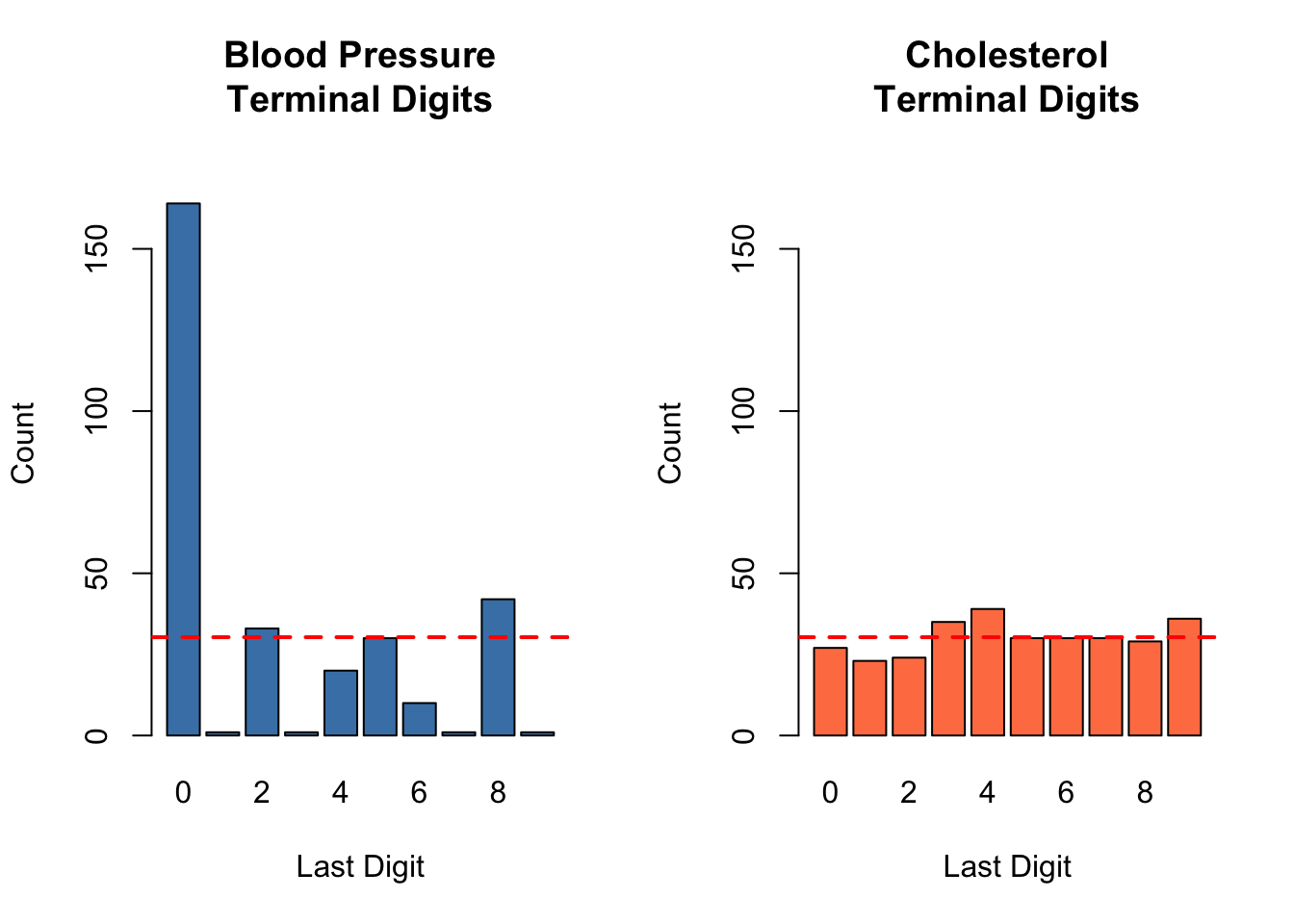
Over half of all blood pressure values (164 out of 303, or 54%) end in the digit 0. The digits 1, 3, 7, and 9 each appear only once. This is a far cry from the expected ~30 observations per digit.
The histogram below shows the terminal digit distribution of blood pressure. Compare the bar heights to the horizontal red line, which marks the expected count under uniformity (~30.3):
The cholesterol terminal digits range from 23 to 39 per digit — much closer to the expected 30.3. The distribution is approximately uniform, as we would expect from a precisely measured continuous variable.
Again, a roughly uniform distribution. The counts range from 17 to 52 — some natural variability, but no single digit dominates.
63.3.5 Why the Difference?
The explanation lies in how each variable was measured:
Blood pressure is measured with a manual sphygmomanometer. A clinician listens for Korotkoff sounds, watches a mercury column, and writes down a number. This process naturally leads to “digit preference” — clinicians tend to round to the nearest 0 or even number.
Cholesterol is measured by an automated laboratory analyser. The machine reports a precise numeric result. There is no human in the loop to introduce rounding.
Max heart rate is recorded by electronic monitoring equipment during an exercise stress test. Again, the machine reports what it measures.
The terminal digit distribution is a “fingerprint” of the measurement process. Manual measurement leaves a distinctive mark; machine measurement does not.
63.4 The “Wrong Tool” Insight
Recall that a frequency table (Chapter 56) is normally used for categorical or discrete data. If we apply it to a truly continuous variable, we expect each value to appear only once or a few times (because, on a continuous scale, the probability of two identical values is essentially zero).
63.4.1 Value Repetition as a Clue
Let us look at the most frequently occurring blood pressure values:
cat("=== Blood Pressure: Top 10 most frequent values ===\n")head(sort(table(heart$bloodpressureNum), decreasing =TRUE), 10)
The most frequent cholesterol value appears only 6 times — exactly what we would expect from a continuously measured variable with 303 observations.
NoteThe Key Insight
If a continuous variable has values appearing 30 or more times out of 303 observations, the measurement process has effectively “discretized” it. A frequency table applied to such data is not “wrong” — it is a diagnostic tool that reveals hidden rounding.
63.5 Even/Odd Asymmetry
The digit preference in blood pressure goes beyond rounding to 0. Let us count even versus odd terminal digits:
=== Blood Pressure ===
Even terminal digits: 269
Odd terminal digits:  34
Ratio (even:odd):     7.9 : 1

=== Cholesterol ===
Even terminal digits: 149
Odd terminal digits:  154
Ratio (even:odd):     1 : 1
Blood pressure has an even-to-odd ratio of about 7.9:1 (269 even vs. 34 odd). Cholesterol has a ratio close to 1:1 (149 even vs. 154 odd). This shows that clinicians do not merely round to the nearest 10 — they prefer all even numbers (0, 2, 4, 6, 8) over odd numbers (1, 3, 5, 7, 9).
63.6 Stem-and-Leaf as Forensic Tool
The stem-and-leaf plot preserves individual digit information (unlike the histogram, which groups values into bins). This makes it a powerful forensic tool. When we display blood pressure as a stem-and-leaf plot, the “leaf” column is dominated by zeros:
stem(heart$bloodpressureNum)
  The decimal point is 1 digit(s) to the right of the |

   9 | 44
  10 | 000012245556888888
  11 | 0000000000000000000222222222455578888888
  12 | 00000000000000000000000000000000000002222344444455555555555666888888
  13 | 00000000000000000000000000000000000022222222444445555556668888888888
  14 | 0000000000000000000000000000000022244555556688
  15 | 0000000000000000022222456
  16 | 0000000000045
  17 | 00002488
  18 | 000
  19 | 2
  20 | 0
Compare with the stem-and-leaf plots in Chapter 61, where the leaves are varied. Here, the repetitive “0” leaves are a visual signature of digit preference.
The strongest evidence comes from a side-by-side comparison. The code below creates barplots of the terminal digit distributions for blood pressure and cholesterol, with a red dashed line marking the expected count under uniformity:
Figure 63.1: Terminal digit distributions of blood pressure (left) and cholesterol (right). The red dashed line marks the expected count under uniformity (n/10 ≈ 30.3). Blood pressure shows extreme digit preference; cholesterol does not.
The contrast is visually striking. The terminal digit distribution is a “forensic fingerprint” that uniquely identifies how a variable was measured.
63.8 Cross-Variable Consistency Check
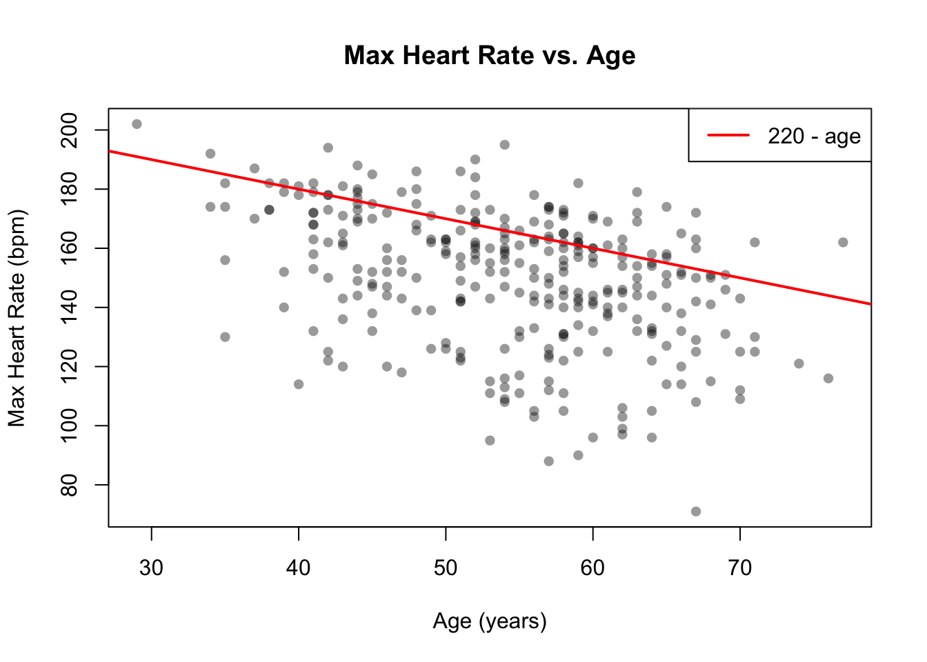
Domain knowledge provides another forensic tool. A widely used rule of thumb states that a person’s maximum heart rate should not exceed approximately \(220 - \text{age}\)(Fox, Naughton, and Haskell 1971). We can check whether the data are consistent with this expectation:
plot(heart$ageNum, heart$maxheartrateNum,xlab ="Age (years)", ylab ="Max Heart Rate (bpm)",main ="Max Heart Rate vs. Age",pch =16, col =rgb(0, 0, 0, 0.4))abline(a =220, b =-1, col ="red", lwd =2)legend("topright", legend ="220 - age", col ="red", lwd =2)# Count points above the lineabove <- heart$maxheartrateNum > (220- heart$ageNum)cat("Patients with max HR above 220 - age:", sum(above), "out of", nrow(heart), "\n")
Patients with max HR above 220 - age: 65 out of 303
Figure 63.2: Maximum heart rate versus age. The solid red line represents the theoretical maximum (220 − age). Points above this line deserve investigation.
A scatterplot is normally used to explore the relationship between two variables (see Chapter 70). Here we use it as a forensic tool: we overlay a domain-knowledge boundary and check for impossible or implausible values. Any observation above the \(220 - \text{age}\) line is worth investigating — it may reflect an unusual patient, a recording error, or the inherent imprecision of the rule of thumb.
63.9 Benford’s Law
63.9.1 Definition
Benford’s Law (Benford 1938; first noted by Newcomb 1881) describes the expected distribution of the first (leading) digit in many naturally occurring datasets. The probability that the first digit is \(d\) (for \(d = 1, 2, \ldots, 9\)) is:
\[P(d) = \log_{10}\left(1 + \frac{1}{d}\right)\]
This gives the following expected distribution:
Digit
1
2
3
4
5
6
7
8
9
Expected %
30.1
17.6
12.5
9.7
7.9
6.7
5.8
5.1
4.6
The key insight is that “1” is the most common leading digit (appearing about 30% of the time), and “9” is the least common (about 4.6%).
63.9.2 When It Applies (and When It Doesn’t)
Benford’s Law works well when the data span multiple orders of magnitude — for example:
Financial transaction amounts (ranging from $1 to $1,000,000)
Population sizes of cities (from hundreds to millions)
River lengths, areas of countries, physical constants
Benford’s Law does not work well when the data are constrained to a narrow range — for example, blood pressure values between 94 and 200, or ages between 29 and 77.
63.9.3 Example: Heart Dataset — A Teaching Moment
Let us compute the first-digit distribution for blood pressure and cholesterol:
first_digit <-function(x) {as.integer(substr(as.character(abs(x)), 1, 1))}benford_expected <-log10(1+1/ (1:9)) *100bp_first <-first_digit(heart$bloodpressureNum)chol_first <-first_digit(heart$cholesterolNum)cat("=== Blood Pressure first digit distribution ===\n")cat("Range:", range(heart$bloodpressureNum), "\n")bp_pct <-round(prop.table(table(factor(bp_first, levels =1:9))) *100, 1)print(bp_pct)cat("\n=== Cholesterol first digit distribution ===\n")cat("Range:", range(heart$cholesterolNum), "\n")chol_pct <-round(prop.table(table(factor(chol_first, levels =1:9))) *100, 1)print(chol_pct)cat("\n=== Benford's Law expected ===\n")cat(round(benford_expected, 1), "\n")
Neither variable follows Benford’s Law well. Blood pressure ranges from 94 to 200, so virtually all first digits are 1. Cholesterol ranges from 126 to 564, concentrating first digits on 1, 2, 3, 4, and 5.
NoteWhen NOT to Apply a Method
Benford’s Law is a powerful forensic tool, but only when the data span several orders of magnitude. Knowing when not to apply a technique is just as important as knowing how to apply it. The heart disease dataset is a useful teaching example precisely because it shows a poor fit.
63.9.4 Where Benford’s Law Shines
As an example of data that do follow Benford’s Law, consider the populations of the world’s countries. These span from a few thousand to over a billion — exactly the kind of data that produces a Benford distribution. Deviations from Benford’s Law in financial data are used as a screening tool for potential fraud or fabrication (Nigrini 1996).
Formal testing of whether an observed digit distribution matches an expected distribution can be done with the chi-squared goodness-of-fit test (Chapter 124).
63.10 Duplicate Detection
Duplicate rows — observations where every variable has the same value — can indicate data entry errors, copy-paste mistakes, or legitimate repeat measurements. Checking for them is a basic data quality step:
Number of exact duplicate rows: 1

Duplicated rows:
    ageNum sexLabel bloodpressureNum cholesterolNum maxheartrateNum
164     38     Male              138            175             173
165     38     Male              138            175             173
When interpreting duplicates, context matters:
In a clinical dataset, two rows with identical values might represent the same patient entered twice (error) or two different patients who happen to share the same measurements (legitimate).
In survey data, exact duplicates are more suspicious because responses tend to vary.
Near-duplicates — rows that match on key columns but differ on others — can also be worth investigating.
63.11 Impossible and Implausible Values
Domain knowledge defines boundaries for what is physically possible and what is merely implausible:
Table 63.1: Domain-knowledge bounds for the heart dataset
Variable
Impossible
Implausible
Systolic blood pressure
< 0 or > 400 mmHg
< 60 or > 250 mmHg
Cholesterol
< 0 mg/dl
< 100 or > 600 mg/dl
Max heart rate
< 0 or > 300 bpm
> 220 for any age
A value of 0 for blood pressure is impossible; a value of 300 is implausible but not impossible in extreme pathology. The distinction matters because impossible values are always errors, while implausible values require judgment.
The forensic techniques in this chapter share a common principle:
If a variable is truly continuous and precisely measured, its terminal digits should be approximately uniformly distributed. Departures from uniformity indicate rounding, digit preference, fabrication, or a discrete measurement process masquerading as continuous.
63.12.1 Purpose
Terminal digit analysis and the related forensic methods can be used to:
Identify data integrity issues (e.g., fabricated data tends to have non-uniform digits because humans are poor random number generators; see Wagenaar (1972))
Validate survey data (e.g., responses that are too “round” may indicate satisficing)
Screen financial data for potential fraud (via Benford’s Law)
63.12.2 Pros & Cons
Pros:
Uses tools students already know (frequency tables, histograms, stem-and-leaf plots)
Extremely simple to compute (only the modulo operator is new)
Detects biases that are invisible to standard descriptive statistics (the mean and standard deviation of blood pressure reveal nothing about digit preference)
Provides visually compelling evidence
Cons:
Requires domain knowledge for interpretation (not all non-uniformity is a problem — for example, age is naturally integer-valued)
Small samples may show non-uniformity by chance alone
Not all non-uniformity indicates an error (blood pressure digit preference reflects how sphygmomanometers work, not a data quality failure)
Diagnostic, not confirmatory — formal testing of digit distributions requires the chi-squared goodness-of-fit test (Chapter 124)
63.13 Example
Using the Histogram app below, you can explore the terminal digit distributions interactively. The data are pre-loaded with the blood pressure terminal digits from the heart dataset. Try changing the number of bins and observe how the digit preference pattern remains visible regardless of binning choices.
Perform terminal digit analysis on bloodpressureMale and bloodpressureFemale separately (these columns contain the blood pressure value for the respective sex and NA for the other). Is digit preference equally severe in both sexes, or does one group show more rounding than the other?
63.14.2 Task 2: Stem-and-Leaf Scale Parameter
Compute stem-and-leaf plots of bloodpressureNum with different values of the scale parameter (try scale = 1 and scale = 2). Which setting makes digit preference more visible? Why?
63.14.3 Task 3: Terminal Digit Analysis of Age
Perform terminal digit analysis on ageNum. Is digit preference present? Should it be present? (Hint: think about how age is recorded.)
63.14.4 Task 4: Cholesterol Digit Distribution
The cholesterol terminal digits are approximately uniform but not perfectly so — digits 4 and 9 appear somewhat more often than others. Is this evidence of digit preference, or could it be due to chance? (Hint: this question can be formally answered with the chi-squared goodness-of-fit test; see Chapter 124.)
63.14.5 Task 5 (Advanced): Benford’s Law in Practice
Find a dataset online with values that span several orders of magnitude (e.g., city populations, financial transaction amounts, or river lengths). Compute the first-digit distribution and compare it to Benford’s Law. Does it fit? Use the chi-squared goodness-of-fit test (Chapter 124) to formally evaluate the fit.
Benford, Frank. 1938. “The Law of Anomalous Numbers.”Proceedings of the American Philosophical Society 78 (4): 551–72.
Fox, Samuel M., John P. Naughton, and William L. Haskell. 1971. “Physical Activity and the Prevention of Coronary Heart Disease.”Annals of Clinical Research 3 (6): 404–32.
Newcomb, Simon. 1881. “Note on the Frequency of Use of the Different Digits in Natural Numbers.”American Journal of Mathematics 4 (1): 39–40. https://doi.org/10.2307/2369148.
Nigrini, Mark J. 1996. A Taxpayer Compliance Application of Benford’s Law. The Journal of the American Taxation Association. Vol. 18. 1.
Wagenaar, Willem A. 1972. “Generation of Random Sequences by Human Subjects: A Critical Survey of the Literature.”Psychological Bulletin 77 (1): 65–72. https://doi.org/10.1037/h0032060.