• Descriptive
    • Moments
    • Concentration
    • Central Tendency
    • Variability
    • Stem-and-Leaf Plot
    • Histogram & Frequency Table
    • Data Quality Forensics
    • Conditional EDA
    • Quantiles
    • Kernel Density Estimation
    • Normal QQ Plot
    • Bootstrap Plot

    • Multivariate Descriptive Statistics
  • Distributions
    • Binomial Probabilities
    • Geometric Probabilities
    • Negative Binomial Probabilities
    • Hypergeometric Probabilities
    • Multinomial Probabilities
    • Dirichlet
    • Poisson Probabilities

    • Exponential
    • Gamma
    • Erlang
    • Weibull
    • Rayleigh
    • Maxwell-Boltzmann
    • Lognormal
    • Pareto
    • Inverse Gamma
    • Inverse Chi-Square

    • Beta
    • Power
    • Beta Prime (Inv. Beta)
    • Triangular

    • Normal (area)
    • Logistic
    • Laplace
    • Cauchy (standard)
    • Cauchy (location-scale)
    • Gumbel
    • Fréchet
    • Generalized Extreme Value

    • Normal RNG
    • ML Fitting
    • Tukey Lambda PPCC
    • Box-Cox Normality Plot
    • Noncentral t
    • Noncentral F
    • Sample Correlation r

    • Empirical Tests
  • Hypotheses
    • Theoretical Aspects of Hypothesis Testing
    • Bayesian Inference
    • Minimum Sample Size

    • Empirical Tests
    • Multivariate (pair-wise) Testing
  • Models
    • Manual Model Building
    • Guided Model Building
  • Time Series
    • Time Series Plot
    • Decomposition
    • Exponential Smoothing

    • Blocked Bootstrap Plot
    • Mean Plot
    • (P)ACF
    • VRM
    • Standard Deviation-Mean Plot
    • Spectral Analysis
    • ARIMA

    • Cross Correlation Function
    • Granger Causality
  1. Probability Distributions
  2. 41  Power Distribution
  • Preface
  • Getting Started
    • 1  Introduction
    • 2  Why Do We Need Innovative Technology?
    • 3  Basic Definitions
    • 4  The Big Picture: Why We Analyze Data
  • Introduction to Probability
    • 5  Definitions of Probability
    • 6  Jeffreys’ axiom system
    • 7  Bayes’ Theorem
    • 8  Sensitivity and Specificity
    • 9  Naive Bayes Classifier
    • 10  Law of Large Numbers

    • 11  Problems
  • Probability Distributions
    • 12  Bernoulli Distribution
    • 13  Binomial Distribution
    • 14  Geometric Distribution
    • 15  Negative Binomial Distribution
    • 16  Hypergeometric Distribution
    • 17  Multinomial Distribution
    • 18  Poisson Distribution

    • 19  Uniform Distribution (Rectangular Distribution)
    • 20  Normal Distribution (Gaussian Distribution)
    • 21  Gaussian Naive Bayes Classifier
    • 22  Chi Distribution
    • 23  Chi-squared Distribution (1 parameter)
    • 24  Chi-squared Distribution (2 parameters)
    • 25  Student t-Distribution
    • 26  Fisher F-Distribution
    • 27  Exponential Distribution
    • 28  Lognormal Distribution
    • 29  Gamma Distribution
    • 30  Beta Distribution
    • 31  Weibull Distribution
    • 32  Pareto Distribution
    • 33  Inverse Gamma Distribution
    • 34  Rayleigh Distribution
    • 35  Erlang Distribution
    • 36  Logistic Distribution
    • 37  Laplace Distribution
    • 38  Gumbel Distribution
    • 39  Cauchy Distribution
    • 40  Triangular Distribution
    • 41  Power Distribution
    • 42  Beta Prime Distribution
    • 43  Sample Correlation Distribution
    • 44  Dirichlet Distribution
    • 45  Generalized Extreme Value (GEV) Distribution
    • 46  Frechet Distribution
    • 47  Noncentral t Distribution
    • 48  Noncentral F Distribution
    • 49  Inverse Chi-Squared Distribution
    • 50  Maxwell-Boltzmann Distribution
    • 51  Distribution Relationship Map

    • 52  Problems
  • Descriptive Statistics & Exploratory Data Analysis
    • 53  Types of Data
    • 54  Datasheets

    • 55  Frequency Plot (Bar Plot)
    • 56  Frequency Table
    • 57  Contingency Table
    • 58  Binomial Classification Metrics
    • 59  Confusion Matrix
    • 60  ROC Analysis

    • 61  Stem-and-Leaf Plot
    • 62  Histogram
    • 63  Data Quality Forensics
    • 64  Quantiles
    • 65  Central Tendency
    • 66  Variability
    • 67  Skewness & Kurtosis
    • 68  Concentration
    • 69  Notched Boxplot
    • 70  Scatterplot
    • 71  Pearson Correlation
    • 72  Rank Correlation
    • 73  Partial Pearson Correlation
    • 74  Simple Linear Regression
    • 75  Moments
    • 76  Quantile-Quantile Plot (QQ Plot)
    • 77  Normal Probability Plot
    • 78  Probability Plot Correlation Coefficient Plot (PPCC Plot)
    • 79  Box-Cox Normality Plot
    • 80  Kernel Density Estimation
    • 81  Bivariate Kernel Density Plot
    • 82  Conditional EDA: Panel Diagnostics
    • 83  Bootstrap Plot (Central Tendency)
    • 84  Survey Scores Rank Order Comparison
    • 85  Cronbach Alpha

    • 86  Equi-distant Time Series
    • 87  Time Series Plot (Run Sequence Plot)
    • 88  Mean Plot
    • 89  Blocked Bootstrap Plot (Central Tendency)
    • 90  Standard Deviation-Mean Plot
    • 91  Variance Reduction Matrix
    • 92  (Partial) Autocorrelation Function
    • 93  Periodogram & Cumulative Periodogram

    • 94  Problems
  • Hypothesis Testing
    • 95  Normal Distributions revisited
    • 96  The Population
    • 97  The Sample
    • 98  The One-Sided Hypothesis Test
    • 99  The Two-Sided Hypothesis Test
    • 100  When to use a one-sided or two-sided test?
    • 101  What if \(\sigma\) is unknown?
    • 102  The Central Limit Theorem (revisited)
    • 103  Statistical Test of the Population Mean with known Variance
    • 104  Statistical Test of the Population Mean with unknown Variance
    • 105  Statistical Test of the Variance
    • 106  Statistical Test of the Population Proportion
    • 107  Statistical Test of the Standard Deviation \(\sigma\)
    • 108  Statistical Test of the difference between Means -- Independent/Unpaired Samples
    • 109  Statistical Test of the difference between Means -- Dependent/Paired Samples
    • 110  Statistical Test of the difference between Variances -- Independent/Unpaired Samples

    • 111  Hypothesis Testing for Research Purposes
    • 112  Decision Thresholds, Alpha, and Confidence Levels
    • 113  Bayesian Inference for Decision-Making
    • 114  One Sample t-Test
    • 115  Skewness & Kurtosis Tests
    • 116  Paired Two Sample t-Test
    • 117  Wilcoxon Signed-Rank Test
    • 118  Unpaired Two Sample t-Test
    • 119  Unpaired Two Sample Welch Test
    • 120  Two One-Sided Tests (TOST) for Equivalence
    • 121  Mann-Whitney U test (Wilcoxon Rank-Sum Test)
    • 122  Bayesian Two Sample Test
    • 123  Median Test based on Notched Boxplots
    • 124  Chi-Squared Tests for Count Data
    • 125  Kolmogorov-Smirnov Test
    • 126  One Way Analysis of Variance (1-way ANOVA)
    • 127  Kruskal-Wallis Test
    • 128  Two Way Analysis of Variance (2-way ANOVA)
    • 129  Repeated Measures ANOVA
    • 130  Friedman Test
    • 131  Testing Correlations
    • 132  A Note on Causality

    • 133  Problems
  • Regression Models
    • 134  Simple Linear Regression Model (SLRM)
    • 135  Multiple Linear Regression Model (MLRM)
    • 136  Logistic Regression
    • 137  Generalized Linear Models
    • 138  Multinomial and Ordinal Logistic Regression
    • 139  Cox Proportional Hazards Regression
    • 140  Conditional Inference Trees
    • 141  Leaf Diagnostics for Conditional Inference Trees
    • 142  Conditional Random Forests
    • 143  Hypothesis Testing with Linear Regression Models (from a Practical Point of View)

    • 144  Problems
  • Introduction to Time Series Analysis
    • 145  Case: the Market of Health and Personal Care Products
    • 146  Decomposition of Time Series
    • 147  Ad hoc Forecasting of Time Series
  • Box-Jenkins Analysis
    • 148  Introduction to Box-Jenkins Analysis
    • 149  Theoretical Concepts
    • 150  Stationarity
    • 151  Identifying ARMA parameters
    • 152  Estimating ARMA Parameters and Residual Diagnostics
    • 153  Forecasting with ARIMA models
    • 154  Intervention Analysis
    • 155  Cross-Correlation Function
    • 156  Transfer Function Noise Models
    • 157  General-to-Specific Modeling
  • Model Building Strategies
    • 158  Introduction to Model Building Strategies
    • 159  Manual Model Building
    • 160  Model Validation
    • 161  Regularization Methods
    • 162  Hyperparameter Optimization Strategies
    • 163  Guided Model Building in Practice
    • 164  Diagnostics, Revision, and Guided Forecasting
    • 165  Leakage, Target Encoding, and Robust Regression
  • References
  • Appendices
    • Appendices
    • A  Method Selection Guide
    • B  Presentations and Teaching Materials
    • C  R Language Concepts for Statistical Computing
    • D  Matrix Algebra
    • E  Standard Normal Table (Gaussian Table)
    • F  Critical values of Student’s \(t\) distribution with \(\nu\) degrees of freedom
    • G  Upper-tail critical values of the \(\chi^2\)-distribution with \(\nu\) degrees of freedom
    • H  Lower-tail critical values of the \(\chi^2\)-distribution with \(\nu\) degrees of freedom

Table of contents

  • 41.1 Probability Density Function
  • 41.2 Purpose
  • 41.3 Distribution Function
  • 41.4 Moment Generating Function
  • 41.5 1st Uncentered Moment
  • 41.6 2nd Uncentered Moment
  • 41.7 3rd Uncentered Moment
  • 41.8 4th Uncentered Moment
  • 41.9 2nd Centered Moment
  • 41.10 3rd Centered Moment
  • 41.11 4th Centered Moment
  • 41.12 Expected Value
  • 41.13 Variance
  • 41.14 Median
  • 41.15 Mode
  • 41.16 Coefficient of Skewness
  • 41.17 Coefficient of Kurtosis
  • 41.18 Parameter Estimation
  • 41.19 R Module
    • 41.19.1 RFC
    • 41.19.2 Direct app link
    • 41.19.3 R Code
  • 41.20 Example
  • 41.21 Random Number Generator
  • 41.22 Property 1: Special Case of Beta
  • 41.23 Property 2: Uniform Special Case
  • 41.24 Property 3: Closed-Form MLE
  • 41.25 Related Distributions 1: Beta Distribution
  • 41.26 Related Distributions 2: Uniform Distribution
  1. Probability Distributions
  2. 41  Power Distribution

41  Power Distribution

The Power distribution is a one-parameter family on \([0,1]\) that generalizes the Uniform distribution. A single shape parameter tilts the density toward 0 (for \(\alpha < 1\)) or toward 1 (for \(\alpha > 1\)), making it useful for bounded quantities with a directional preference.

Formally, the random variate \(X\) defined for the range \(X \in [0, 1]\), is said to have a Power Distribution (i.e. \(X \sim \text{Power}(\alpha)\)) with shape parameter \(\alpha > 0\). The Power distribution is equivalent to Beta\((\alpha, 1)\).

41.1 Probability Density Function

\[ f(x) = \alpha\, x^{\alpha-1}, \quad 0 \leq x \leq 1 \]

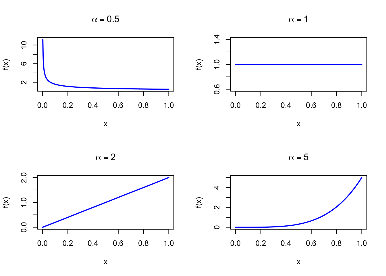
The figure below shows examples of the Power Probability Density Function for different shape values.

Code
par(mfrow = c(2, 2))
x <- seq(0, 1, length = 500)

plot(x, dbeta(x, shape1 = 0.5, shape2 = 1), type = "l", lwd = 2, col = "blue",
     xlab = "x", ylab = "f(x)", main = expression(alpha == 0.5))

plot(x, dbeta(x, shape1 = 1, shape2 = 1), type = "l", lwd = 2, col = "blue",
     xlab = "x", ylab = "f(x)", main = expression(alpha == 1))

plot(x, dbeta(x, shape1 = 2, shape2 = 1), type = "l", lwd = 2, col = "blue",
     xlab = "x", ylab = "f(x)", main = expression(alpha == 2))

plot(x, dbeta(x, shape1 = 5, shape2 = 1), type = "l", lwd = 2, col = "blue",
     xlab = "x", ylab = "f(x)", main = expression(alpha == 5))

par(mfrow = c(1, 1))
Figure 41.1: Power Probability Density Function for various shape values

41.2 Purpose

The Power distribution models bounded quantities in \([0,1]\) when the density is monotone — either increasing or decreasing — rather than bell-shaped. Its single parameter determines whether small values (near 0) or large values (near 1) are most likely. Common applications include:

  • Proportion of correct answers when most respondents score high or low
  • Reliability: proportion of items surviving a stress test when failure is rare or common
  • Revenue share distributions: when one party captures most of the total
  • Prior distribution for probabilities biased toward extreme values
  • Order statistics from the Uniform distribution on \([0,1]\)

Relation to the discrete setting. Power\((\alpha)\) = Beta\((\alpha, 1)\) is a continuous model for proportions; its discrete analog is the Bernoulli distribution (for a single bounded outcome) or a Discrete Uniform (when \(\alpha = 1\)). For integer-valued bounded counts, the Binomial plays a similar role.

41.3 Distribution Function

\[ F(x) = x^\alpha, \quad 0 \leq x \leq 1 \]

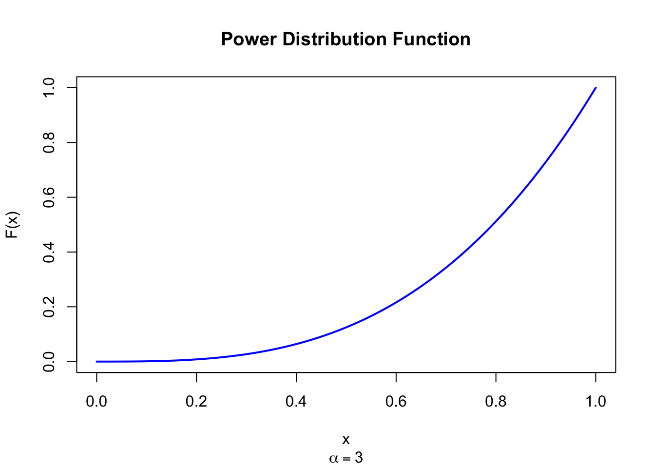
The figure below shows the Power Distribution Function for \(\alpha = 3\).

Code
x <- seq(0, 1, length = 500)
plot(x, pbeta(x, shape1 = 3, shape2 = 1), type = "l", lwd = 2, col = "blue",
     xlab = "x", ylab = "F(x)", main = "Power Distribution Function",
     sub = expression(alpha == 3))
Figure 41.2: Power Distribution Function (alpha = 3)

41.4 Moment Generating Function

The MGF has no simple closed form. Raw moments are computed directly:

\[ \mu_n' = \frac{\alpha}{\alpha + n} \]

41.5 1st Uncentered Moment

\[ \mu_1' = \frac{\alpha}{\alpha + 1} \]

41.6 2nd Uncentered Moment

\[ \mu_2' = \frac{\alpha}{\alpha + 2} \]

41.7 3rd Uncentered Moment

\[ \mu_3' = \frac{\alpha}{\alpha + 3} \]

41.8 4th Uncentered Moment

\[ \mu_4' = \frac{\alpha}{\alpha + 4} \]

41.9 2nd Centered Moment

\[ \mu_2 = \frac{\alpha}{(\alpha+1)^2(\alpha+2)} \]

41.10 3rd Centered Moment

\[ \mu_3 = \frac{2\alpha(1-\alpha)}{(\alpha+1)^3(\alpha+2)(\alpha+3)} \]

41.11 4th Centered Moment

Obtained by expanding from raw moments.

41.12 Expected Value

\[ \text{E}(X) = \frac{\alpha}{\alpha + 1} \]

41.13 Variance

\[ \text{V}(X) = \frac{\alpha}{(\alpha+1)^2(\alpha+2)} \]

41.14 Median

\[ \text{Med}(X) = 2^{-1/\alpha} \]

41.15 Mode

\[ \text{Mo}(X) = \begin{cases} 1 & \alpha > 1 \\ 0 & \alpha < 1 \\ \text{any value in } [0,1] & \alpha = 1 \end{cases} \]

41.16 Coefficient of Skewness

\[ g_1 = \frac{2(1-\alpha)\sqrt{\alpha+2}}{(\alpha+3)\sqrt{\alpha}} \]

For \(\alpha = 1\): \(g_1 = 0\) (Uniform is symmetric). For \(\alpha > 1\): \(g_1 < 0\) (left-skewed toward 1).

41.17 Coefficient of Kurtosis

\[ g_2 = 3 + \frac{6(\alpha^3 - \alpha^2 - 2\alpha - 2)}{\alpha(\alpha+3)(\alpha+4)} \]

At \(\alpha = 1\) (Uniform): \(g_2 = 3 + 6(1-1-2-2)/(1\cdot 4\cdot 5) = 3 - 24/20 = 3 - 1.2 = 1.8\). ✓

41.18 Parameter Estimation

The MLE has a rare closed form:

\[ \hat\alpha = -\frac{n}{\displaystyle\sum_{i=1}^n \ln x_i} \]

set.seed(42)
alpha_true <- 3
x_obs <- rbeta(100, shape1 = alpha_true, shape2 = 1)

# MLE
alpha_hat <- -length(x_obs) / sum(log(x_obs))
cat("MLE alpha:", round(alpha_hat, 4), "\n")
cat("True alpha:", alpha_true, "\n")

# Mean comparison
cat("MLE mean:", alpha_hat / (alpha_hat + 1), "\n")
cat("Sample mean:", mean(x_obs), "\n")
MLE alpha: 2.9641 
True alpha: 3 
MLE mean: 0.7477371 
Sample mean: 0.7450839 

41.19 R Module

41.19.1 RFC

The Power Distribution module is available in RFC under the menu “Distributions / Power Distribution”.

41.19.2 Direct app link

  • https://shiny.wessa.net/power/

41.19.3 R Code

The following code demonstrates Power distribution probability calculations using dbeta/pbeta with shape2 = 1:

alpha <- 3

# Using Beta(alpha, 1) equivalence
dbeta(0.75, shape1 = alpha, shape2 = 1)

# P(X <= 0.75)
pbeta(0.75, shape1 = alpha, shape2 = 1)

# Median
cat("Median:", 2^(-1/alpha), "\n")

# Mean
cat("Mean:", alpha / (alpha + 1), "\n")
[1] 1.6875
[1] 0.421875
Median: 0.7937005 
Mean: 0.75 

41.20 Example

The proportion of correct answers on a test is modeled as \(X \sim \text{Power}(3)\). This implies the density is \(f(x) = 3x^2\), concentrated toward high scores. The mean proportion is \(3/4 = 0.75\).

alpha <- 3

# P(proportion <= 0.75)
cat("P(score proportion <= 0.75):", pbeta(0.75, alpha, 1), "\n")

# Mean and median
cat("Mean:", alpha / (alpha + 1), "\n")
cat("Median:", round(2^(-1/alpha), 4), "\n")

# Skewness (negative = left-skewed toward 1)
g1 <- 2 * (1 - alpha) * sqrt(alpha + 2) / ((alpha + 3) * sqrt(alpha))
cat("Skewness g1:", round(g1, 4), "\n")
P(score proportion <= 0.75): 0.421875 
Mean: 0.75 
Median: 0.7937 
Skewness g1: -0.8607 
Interactive Shiny app (click to load).
Open in new tab

41.21 Random Number Generator

The Power distribution has the simplest possible random number generator via the inverse-CDF. Since \(F(x) = x^\alpha\):

\[ X = U^{1/\alpha} \sim \text{Power}(\alpha) \quad \text{when } U \sim \text{U}(0,1) \]

set.seed(123)
n <- 1000; alpha <- 3

# Inverse-transform method
u <- runif(n)
x_inv <- u^(1/alpha)

cat("Simulated mean:", round(mean(x_inv), 4), "\n")
cat("Theoretical mean:", alpha / (alpha + 1), "\n")
cat("Simulated var:", round(var(x_inv), 4), "\n")
cat("Theoretical var:", alpha / ((alpha+1)^2 * (alpha+2)), "\n")
Simulated mean: 0.7487 
Theoretical mean: 0.75 
Simulated var: 0.0374 
Theoretical var: 0.0375 
Interactive Shiny app (click to load).
Open in new tab

41.22 Property 1: Special Case of Beta

The Power distribution is the Beta distribution with shape parameters \((\alpha, 1)\):

\[ \text{Power}(\alpha) = \text{Beta}(\alpha, 1) \]

All Beta distribution properties apply, and R’s dbeta, pbeta, qbeta, and rbeta with shape2 = 1 compute the Power distribution exactly. See Chapter 30.

41.23 Property 2: Uniform Special Case

When \(\alpha = 1\), the Power distribution reduces to the Uniform\((0, 1)\) distribution:

\[ \text{Power}(1) = \text{U}(0, 1) \]

See Chapter 19.

41.24 Property 3: Closed-Form MLE

The MLE \(\hat\alpha = -n/\sum \ln x_i\) is one of the few analytically tractable maximum likelihood estimators in the Beta family, but it is biased for \(n > 1\). For \(n > 1\), the UMVUE is \(\hat\alpha_U = (n-1)/(-\sum \ln x_i)\).

41.25 Related Distributions 1: Beta Distribution

The Power distribution is the Beta\((\alpha, 1)\) special case (see Chapter 30).

41.26 Related Distributions 2: Uniform Distribution

The Uniform distribution is Power\((1)\) (see Chapter 19).

40  Triangular Distribution
42  Beta Prime Distribution

© 2026 Patrick Wessa. Provided as-is, without warranty.

Feedback: e-mail | Anonymous contributions: click to copy (Sats) | click to copy (XMR)

Cookie Preferences