49  Inverse Chi-Squared Distribution

The Scaled Inverse Chi-Squared distribution is the standard conjugate prior for the variance parameter \(\sigma^2\) of a Normal distribution in Bayesian inference. It arises whenever one models uncertainty about a variance or scale parameter, and its posterior updating rules are analytically tractable.

Formally, the random variate \(X\) defined for the range \(X > 0\), is said to have a Scaled Inverse Chi-Squared Distribution (i.e. \(X \sim \text{Inv-}\chi^2(\nu, \tau^2)\)) with degrees of freedom \(\nu > 0\) and scale parameter \(\tau^2 > 0\). The Scaled Inverse Chi-Squared distribution is a special case of the Inverse Gamma distribution: \(\text{Inv-}\chi^2(\nu, \tau^2) = \text{InvGamma}(\nu/2,\, \nu\tau^2/2)\).

49.1 Probability Density Function

\[ f(x) = \frac{(\nu\tau^2/2)^{\nu/2}}{\Gamma(\nu/2)}\,x^{-\nu/2-1}\exp\!\left(-\frac{\nu\tau^2}{2x}\right), \quad x > 0 \]

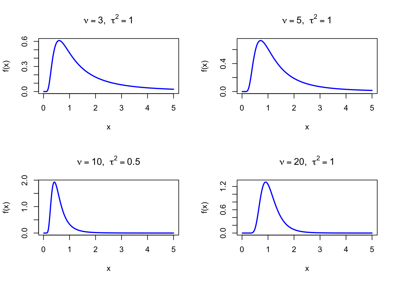
The figure below shows examples of the Scaled Inverse Chi-Squared Probability Density Function for different parameter combinations.

dinvchisq <- function(x, nu, tau2) {
  a <- nu / 2
  b <- nu * tau2 / 2
  ifelse(x > 0, b^a / gamma(a) * x^(-a - 1) * exp(-b / x), 0)
}

par(mfrow = c(2, 2))
x <- seq(0.01, 5, length = 500)

plot(x, dinvchisq(x, 3, 1), type = "l", lwd = 2, col = "blue",
     xlab = "x", ylab = "f(x)", main = expression(paste(nu == 3, ",  ", tau^2 == 1)))

plot(x, dinvchisq(x, 5, 1), type = "l", lwd = 2, col = "blue",
     xlab = "x", ylab = "f(x)", main = expression(paste(nu == 5, ",  ", tau^2 == 1)))

plot(x, dinvchisq(x, 10, 0.5), type = "l", lwd = 2, col = "blue",
     xlab = "x", ylab = "f(x)", main = expression(paste(nu == 10, ",  ", tau^2 == 0.5)))

plot(x, dinvchisq(x, 20, 1), type = "l", lwd = 2, col = "blue",
     xlab = "x", ylab = "f(x)", main = expression(paste(nu == 20, ",  ", tau^2 == 1)))

par(mfrow = c(1, 1))

Figure 49.1: Scaled Inverse Chi-Squared Probability Density Function for various parameter combinations

49.2 Purpose

The Scaled Inverse Chi-Squared distribution is the workhorse prior for variance parameters in Bayesian statistics. Its closed-form posterior updating rules make it indispensable for conjugate analysis of Normal models. Common applications include:

• Conjugate prior for the variance \(\sigma^2\) in Normal-Normal models
• Posterior distribution of variance after observing Gaussian data with known mean
• Hierarchical models where group-level variances require a prior
• Objective Bayesian analysis (Jeffreys prior for variance corresponds to \(\nu = 0\), \(\tau^2 = 0\))
• Uncertainty quantification for measurement precision and instrument calibration

Relation to the Inverse Gamma. The Scaled Inverse Chi-Squared distribution is a reparameterization of the Inverse Gamma: \(\text{Inv-}\chi^2(\nu, \tau^2) = \text{InvGamma}(\nu/2,\, \nu\tau^2/2)\). The \((\nu, \tau^2)\) parameterization has a natural interpretation in Bayesian inference — \(\nu\) represents the prior sample size and \(\tau^2\) represents the prior estimate of the variance.

49.3 Distribution Function

\[ F(x) = \frac{\Gamma(\nu/2,\, \nu\tau^2/(2x))}{\Gamma(\nu/2)}, \quad x > 0 \]

where \(\Gamma(\alpha, z) = \int_z^\infty t^{\alpha-1} e^{-t}\, dt\) is the upper incomplete gamma function. In R: pgamma(1/x, shape = nu/2, rate = nu*tau2/2, lower.tail = FALSE).

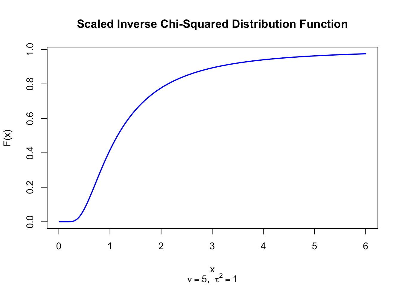
The figure below shows the Scaled Inverse Chi-Squared Distribution Function for \(\nu = 5\) and \(\tau^2 = 1\).

pinvchisq <- function(x, nu, tau2) {
  pgamma(1/x, shape = nu/2, rate = nu * tau2 / 2, lower.tail = FALSE)
}

x <- seq(0.01, 6, length = 500)
plot(x, pinvchisq(x, 5, 1), type = "l", lwd = 2, col = "blue",
     xlab = "x", ylab = "F(x)", main = "Scaled Inverse Chi-Squared Distribution Function",
     sub = expression(paste(nu == 5, ",  ", tau^2 == 1)))

Figure 49.2: Scaled Inverse Chi-Squared Distribution Function (nu = 5, tau^2 = 1)

49.4 Moment Generating Function

The moment generating function of the Scaled Inverse Chi-Squared distribution does not exist for \(t > 0\).

49.5 Expected Value

\[ \text{E}(X) = \frac{\nu\tau^2}{\nu - 2}, \quad \nu > 2 \]

The mean is undefined for \(\nu \leq 2\).

49.6 Variance

\[ \text{V}(X) = \frac{2\nu^2\tau^4}{(\nu-2)^2(\nu-4)}, \quad \nu > 4 \]

49.7 Median

The median has no closed form and must be computed numerically:

# Median of Inv-Chi-sq(nu, tau2): numerical
nu <- 5; tau2 <- 1
pinvchisq <- function(x, nu, tau2) pgamma(1/x, shape = nu/2, rate = nu * tau2 / 2, lower.tail = FALSE)
uniroot(function(x) pinvchisq(x, nu, tau2) - 0.5, c(0.001, 1000))$root

[1] 1.14904

49.8 Mode

\[ \text{Mo}(X) = \frac{\nu\tau^2}{\nu + 2} \]

49.9 Coefficient of Skewness

\[ g_1 = \frac{4\sqrt{2(\nu - 4)}}{\nu - 6}, \quad \nu > 6 \]

The Scaled Inverse Chi-Squared distribution is always positively skewed. The skewness decreases as \(\nu\) increases, reflecting a more symmetric shape for larger degrees of freedom.

49.10 Coefficient of Kurtosis

\[ g_2 = 3 + \frac{12(5\nu - 22)}{(\nu-6)(\nu-8)}, \quad \nu > 8 \]

The excess kurtosis \(g_2 - 3 = \frac{12(5\nu - 22)}{(\nu-6)(\nu-8)}\) is always positive, indicating heavier tails than the Normal distribution.

49.11 Parameter Estimation

Since \(\text{Inv-}\chi^2(\nu, \tau^2) = \text{InvGamma}(\nu/2,\, \nu\tau^2/2)\), parameter estimation is performed by first estimating the Inverse Gamma parameters \(\alpha\) and \(\beta\) and then recovering \(\nu = 2\alpha\) and \(\tau^2 = \beta/\alpha\). Method-of-moments starting values from the Inverse Gamma parameterization:

\[ \tilde\alpha = \frac{\bar x^2}{s^2} + 2, \qquad \tilde\beta = \bar x\,(\tilde\alpha - 1) \]

then \(\tilde\nu = 2\tilde\alpha\) and \(\tilde\tau^2 = \tilde\beta / \tilde\alpha\).

# Simulate Inv-Chi-sq(10, 1) data and estimate parameters
set.seed(42)
nu_true <- 10; tau2_true <- 1

# Inv-Chi-sq(nu, tau2) = InvGamma(nu/2, nu*tau2/2)
alpha_true <- nu_true / 2
beta_true  <- nu_true * tau2_true / 2
x_sim <- 1 / rgamma(200, shape = alpha_true, rate = beta_true)

# Method-of-moments starting values (Inverse Gamma)
xbar <- mean(x_sim); s2 <- var(x_sim)
alpha_mom <- xbar^2 / s2 + 2
beta_mom  <- xbar * (alpha_mom - 1)
nu_mom    <- 2 * alpha_mom
tau2_mom  <- beta_mom / alpha_mom

cat("MoM nu:", round(nu_mom, 4), "  MoM tau^2:", round(tau2_mom, 4), "\n")
cat("True nu:", nu_true, "  True tau^2:", tau2_true, "\n")

MoM nu: 7.3319   MoM tau^2: 0.9623 
True nu: 10   True tau^2: 1 

49.12 R Module

49.12.1 RFC

The Inverse Chi-Squared Distribution module is available in RFC under the menu “Distributions / Inverse Chi-Squared Distribution”.

49.12.2 Direct app link

• https://shiny.wessa.net/invchisq/

49.12.3 R Code

The following code demonstrates Scaled Inverse Chi-Squared probability calculations:

nu <- 5; tau2 <- 1

# Custom density function
dinvchisq <- function(x, nu, tau2) {
  a <- nu / 2; b <- nu * tau2 / 2
  ifelse(x > 0, b^a / gamma(a) * x^(-a - 1) * exp(-b / x), 0)
}

# Custom CDF using pgamma
pinvchisq <- function(x, nu, tau2) {
  pgamma(1/x, shape = nu/2, rate = nu * tau2 / 2, lower.tail = FALSE)
}

# Density at x = 1
dinvchisq(1, nu, tau2)

# P(X <= 1): distribution function
pinvchisq(1, nu, tau2)

# Mode and mean
cat("Mode:", nu * tau2 / (nu + 2), "\n")
cat("Mean:", nu * tau2 / (nu - 2), "\n")

[1] 0.6102076
[1] 0.4158802
Mode: 0.7142857 
Mean: 1.666667 

49.13 Example

A Bayesian analyst places a \(\text{Inv-}\chi^2(\nu_0 = 5,\, \tau_0^2 = 1)\) prior on the variance \(\sigma^2\) of a Normal likelihood. This prior represents a belief that \(\sigma^2\) is around 1, supported by the equivalent of 5 prior observations. After observing \(n = 20\) data points from \(N(\mu, \sigma^2)\) with known mean \(\mu\) and sum of squared errors \(\text{SSE} = 18\), the posterior is:

\[ \sigma^2 \mid \mathbf{x} \sim \text{Inv-}\chi^2\!\left(\nu_0 + n,\; \frac{\nu_0\tau_0^2 + \text{SSE}}{\nu_0 + n}\right) \]

# Prior parameters
nu0 <- 5; tau0_sq <- 1

# Observed data summary
n <- 20; SSE <- 18

# Posterior parameters
nu_post  <- nu0 + n
tau2_post <- (nu0 * tau0_sq + SSE) / (nu0 + n)

cat("Posterior nu:", nu_post, "\n")
cat("Posterior tau^2:", round(tau2_post, 4), "\n")
cat("Posterior mean:", round(nu_post * tau2_post / (nu_post - 2), 4), "\n")
cat("Posterior mode:", round(nu_post * tau2_post / (nu_post + 2), 4), "\n")

# 95% credible interval
pinvchisq <- function(x, nu, tau2) {
  pgamma(1/x, shape = nu/2, rate = nu * tau2 / 2, lower.tail = FALSE)
}
qinvchisq <- function(p, nu, tau2) {
  1 / qgamma(1 - p, shape = nu/2, rate = nu * tau2 / 2)
}

lower <- qinvchisq(0.025, nu_post, tau2_post)
upper <- qinvchisq(0.975, nu_post, tau2_post)
cat("95% credible interval: [", round(lower, 4), ",", round(upper, 4), "]\n")

Posterior nu: 25 
Posterior tau^2: 0.92 
Posterior mean: 1 
Posterior mode: 0.8519 
95% credible interval: [ 0.5659 , 1.7531 ]

Interactive Shiny app (click to load).

Open in new tab

49.14 Random Number Generator

Scaled Inverse Chi-Squared random variates are generated as reciprocals of Gamma variates, using the equivalence with the Inverse Gamma distribution:

\[ \text{If } Y \sim \text{Gamma}(\nu/2,\, \nu\tau^2/2) \text{ then } X = 1/Y \sim \text{Inv-}\chi^2(\nu, \tau^2) \]

set.seed(123)
n <- 1000
nu <- 10; tau2 <- 1

# Generate Inv-Chi-sq via reciprocal of Gamma
y <- rgamma(n, shape = nu/2, rate = nu * tau2 / 2)
x_sim <- 1 / y

cat("Simulated mean:", round(mean(x_sim), 4), "\n")
cat("Theoretical mean:", nu * tau2 / (nu - 2), "\n")
cat("Simulated var:", round(var(x_sim), 4), "\n")
cat("Theoretical var:", 2 * nu^2 * tau2^2 / ((nu-2)^2 * (nu-4)), "\n")

Simulated mean: 1.2773 
Theoretical mean: 1.25 
Simulated var: 0.468 
Theoretical var: 0.5208333 

Interactive Shiny app (click to load).

Open in new tab

49.15 Property 1: Special Case of the Inverse Gamma

The Scaled Inverse Chi-Squared distribution is a reparameterization of the Inverse Gamma distribution:

\[ \text{Inv-}\chi^2(\nu, \tau^2) = \text{InvGamma}\!\left(\frac{\nu}{2},\, \frac{\nu\tau^2}{2}\right) \]

See Chapter 33.

49.16 Property 2: Conjugate Prior for Normal Variance

If \(X_1, \ldots, X_n \overset{\text{i.i.d.}}{\sim} N(\mu, \sigma^2)\) with known mean \(\mu\) and \(\sigma^2 \sim \text{Inv-}\chi^2(\nu_0, \tau_0^2)\), then the posterior distribution of \(\sigma^2\) is:

\[ \sigma^2 \mid \mathbf{x} \sim \text{Inv-}\chi^2\!\left(\nu_0 + n,\; \frac{\nu_0\tau_0^2 + \text{SSE}}{\nu_0 + n}\right) \]

where \(\text{SSE} = \sum_{i=1}^n (x_i - \mu)^2\). The posterior degrees of freedom \(\nu_0 + n\) accumulate the prior and data information, while the posterior scale \(\tau_{\text{post}}^2\) is a weighted average of the prior scale and the data-driven variance estimate. See Chapter 20.

49.17 Property 3: Reciprocal of Chi-Squared

If \(Y \sim \chi^2(\nu)\) then \(1/Y\) follows an (unscaled) Inverse Chi-Squared distribution. The scaled version adds a scale factor:

\[ \text{If } Y \sim \chi^2(\nu) \text{ then } \frac{\nu\tau^2}{Y} \sim \text{Inv-}\chi^2(\nu, \tau^2) \]

See Chapter 23.

49.18 Property 4: Jeffreys Prior Limit

As \(\nu \to 0\) and \(\tau^2 \to 0\), the Scaled Inverse Chi-Squared prior becomes the Jeffreys noninformative prior for variance, \(p(\sigma^2) \propto 1/\sigma^2\). This limiting form is widely used in objective Bayesian analysis.

49.19 Related Distributions 1: Inverse Gamma Distribution

The Inverse Gamma distribution is the general two-parameter family of which the Scaled Inverse Chi-Squared is a special case: \(\text{Inv-}\chi^2(\nu, \tau^2) = \text{InvGamma}(\nu/2,\, \nu\tau^2/2)\) (see Chapter 33).

49.20 Related Distributions 2: Chi-Squared Distribution

The Chi-Squared distribution with \(\nu\) degrees of freedom is related through the reciprocal transformation: if \(Y \sim \chi^2(\nu)\) then \(\nu\tau^2 / Y \sim \text{Inv-}\chi^2(\nu, \tau^2)\) (see Chapter 23).

49.21 Related Distributions 3: Normal Distribution

The Scaled Inverse Chi-Squared distribution serves as the conjugate prior for the variance \(\sigma^2\) of a Normal likelihood. The Normal-Inverse-Chi-Squared model is a fundamental building block of Bayesian inference (see Chapter 20).