• Descriptive
    • Moments
    • Concentration
    • Central Tendency
    • Variability
    • Stem-and-Leaf Plot
    • Histogram & Frequency Table
    • Data Quality Forensics
    • Conditional EDA
    • Quantiles
    • Kernel Density Estimation
    • Normal QQ Plot
    • Bootstrap Plot

    • Multivariate Descriptive Statistics
  • Distributions
    • Binomial Probabilities
    • Geometric Probabilities
    • Negative Binomial Probabilities
    • Hypergeometric Probabilities
    • Multinomial Probabilities
    • Dirichlet
    • Poisson Probabilities

    • Exponential
    • Gamma
    • Erlang
    • Weibull
    • Rayleigh
    • Maxwell-Boltzmann
    • Lognormal
    • Pareto
    • Inverse Gamma
    • Inverse Chi-Square

    • Beta
    • Power
    • Beta Prime (Inv. Beta)
    • Triangular

    • Normal (area)
    • Logistic
    • Laplace
    • Cauchy (standard)
    • Cauchy (location-scale)
    • Gumbel
    • Fréchet
    • Generalized Extreme Value

    • Normal RNG
    • ML Fitting
    • Tukey Lambda PPCC
    • Box-Cox Normality Plot
    • Noncentral t
    • Noncentral F
    • Sample Correlation r

    • Empirical Tests
  • Hypotheses
    • Theoretical Aspects of Hypothesis Testing
    • Bayesian Inference
    • Minimum Sample Size

    • Empirical Tests
    • Multivariate (pair-wise) Testing
  • Models
    • Manual Model Building
    • Guided Model Building
  • Time Series
    • Time Series Plot
    • Decomposition
    • Exponential Smoothing

    • Blocked Bootstrap Plot
    • Mean Plot
    • (P)ACF
    • VRM
    • Standard Deviation-Mean Plot
    • Spectral Analysis
    • ARIMA

    • Cross Correlation Function
    • Granger Causality
  1. Probability Distributions
  2. 35  Erlang Distribution
  • Preface
  • Getting Started
    • 1  Introduction
    • 2  Why Do We Need Innovative Technology?
    • 3  Basic Definitions
    • 4  The Big Picture: Why We Analyze Data
  • Introduction to Probability
    • 5  Definitions of Probability
    • 6  Jeffreys’ axiom system
    • 7  Bayes’ Theorem
    • 8  Sensitivity and Specificity
    • 9  Naive Bayes Classifier
    • 10  Law of Large Numbers

    • 11  Problems
  • Probability Distributions
    • 12  Bernoulli Distribution
    • 13  Binomial Distribution
    • 14  Geometric Distribution
    • 15  Negative Binomial Distribution
    • 16  Hypergeometric Distribution
    • 17  Multinomial Distribution
    • 18  Poisson Distribution

    • 19  Uniform Distribution (Rectangular Distribution)
    • 20  Normal Distribution (Gaussian Distribution)
    • 21  Gaussian Naive Bayes Classifier
    • 22  Chi Distribution
    • 23  Chi-squared Distribution (1 parameter)
    • 24  Chi-squared Distribution (2 parameters)
    • 25  Student t-Distribution
    • 26  Fisher F-Distribution
    • 27  Exponential Distribution
    • 28  Lognormal Distribution
    • 29  Gamma Distribution
    • 30  Beta Distribution
    • 31  Weibull Distribution
    • 32  Pareto Distribution
    • 33  Inverse Gamma Distribution
    • 34  Rayleigh Distribution
    • 35  Erlang Distribution
    • 36  Logistic Distribution
    • 37  Laplace Distribution
    • 38  Gumbel Distribution
    • 39  Cauchy Distribution
    • 40  Triangular Distribution
    • 41  Power Distribution
    • 42  Beta Prime Distribution
    • 43  Sample Correlation Distribution
    • 44  Dirichlet Distribution
    • 45  Generalized Extreme Value (GEV) Distribution
    • 46  Frechet Distribution
    • 47  Noncentral t Distribution
    • 48  Noncentral F Distribution
    • 49  Inverse Chi-Squared Distribution
    • 50  Maxwell-Boltzmann Distribution
    • 51  Distribution Relationship Map

    • 52  Problems
  • Descriptive Statistics & Exploratory Data Analysis
    • 53  Types of Data
    • 54  Datasheets

    • 55  Frequency Plot (Bar Plot)
    • 56  Frequency Table
    • 57  Contingency Table
    • 58  Binomial Classification Metrics
    • 59  Confusion Matrix
    • 60  ROC Analysis

    • 61  Stem-and-Leaf Plot
    • 62  Histogram
    • 63  Data Quality Forensics
    • 64  Quantiles
    • 65  Central Tendency
    • 66  Variability
    • 67  Skewness & Kurtosis
    • 68  Concentration
    • 69  Notched Boxplot
    • 70  Scatterplot
    • 71  Pearson Correlation
    • 72  Rank Correlation
    • 73  Partial Pearson Correlation
    • 74  Simple Linear Regression
    • 75  Moments
    • 76  Quantile-Quantile Plot (QQ Plot)
    • 77  Normal Probability Plot
    • 78  Probability Plot Correlation Coefficient Plot (PPCC Plot)
    • 79  Box-Cox Normality Plot
    • 80  Kernel Density Estimation
    • 81  Bivariate Kernel Density Plot
    • 82  Conditional EDA: Panel Diagnostics
    • 83  Bootstrap Plot (Central Tendency)
    • 84  Survey Scores Rank Order Comparison
    • 85  Cronbach Alpha

    • 86  Equi-distant Time Series
    • 87  Time Series Plot (Run Sequence Plot)
    • 88  Mean Plot
    • 89  Blocked Bootstrap Plot (Central Tendency)
    • 90  Standard Deviation-Mean Plot
    • 91  Variance Reduction Matrix
    • 92  (Partial) Autocorrelation Function
    • 93  Periodogram & Cumulative Periodogram

    • 94  Problems
  • Hypothesis Testing
    • 95  Normal Distributions revisited
    • 96  The Population
    • 97  The Sample
    • 98  The One-Sided Hypothesis Test
    • 99  The Two-Sided Hypothesis Test
    • 100  When to use a one-sided or two-sided test?
    • 101  What if \(\sigma\) is unknown?
    • 102  The Central Limit Theorem (revisited)
    • 103  Statistical Test of the Population Mean with known Variance
    • 104  Statistical Test of the Population Mean with unknown Variance
    • 105  Statistical Test of the Variance
    • 106  Statistical Test of the Population Proportion
    • 107  Statistical Test of the Standard Deviation \(\sigma\)
    • 108  Statistical Test of the difference between Means -- Independent/Unpaired Samples
    • 109  Statistical Test of the difference between Means -- Dependent/Paired Samples
    • 110  Statistical Test of the difference between Variances -- Independent/Unpaired Samples

    • 111  Hypothesis Testing for Research Purposes
    • 112  Decision Thresholds, Alpha, and Confidence Levels
    • 113  Bayesian Inference for Decision-Making
    • 114  One Sample t-Test
    • 115  Skewness & Kurtosis Tests
    • 116  Paired Two Sample t-Test
    • 117  Wilcoxon Signed-Rank Test
    • 118  Unpaired Two Sample t-Test
    • 119  Unpaired Two Sample Welch Test
    • 120  Two One-Sided Tests (TOST) for Equivalence
    • 121  Mann-Whitney U test (Wilcoxon Rank-Sum Test)
    • 122  Bayesian Two Sample Test
    • 123  Median Test based on Notched Boxplots
    • 124  Chi-Squared Tests for Count Data
    • 125  Kolmogorov-Smirnov Test
    • 126  One Way Analysis of Variance (1-way ANOVA)
    • 127  Kruskal-Wallis Test
    • 128  Two Way Analysis of Variance (2-way ANOVA)
    • 129  Repeated Measures ANOVA
    • 130  Friedman Test
    • 131  Testing Correlations
    • 132  A Note on Causality

    • 133  Problems
  • Regression Models
    • 134  Simple Linear Regression Model (SLRM)
    • 135  Multiple Linear Regression Model (MLRM)
    • 136  Logistic Regression
    • 137  Generalized Linear Models
    • 138  Multinomial and Ordinal Logistic Regression
    • 139  Cox Proportional Hazards Regression
    • 140  Conditional Inference Trees
    • 141  Leaf Diagnostics for Conditional Inference Trees
    • 142  Conditional Random Forests
    • 143  Hypothesis Testing with Linear Regression Models (from a Practical Point of View)

    • 144  Problems
  • Introduction to Time Series Analysis
    • 145  Case: the Market of Health and Personal Care Products
    • 146  Decomposition of Time Series
    • 147  Ad hoc Forecasting of Time Series
  • Box-Jenkins Analysis
    • 148  Introduction to Box-Jenkins Analysis
    • 149  Theoretical Concepts
    • 150  Stationarity
    • 151  Identifying ARMA parameters
    • 152  Estimating ARMA Parameters and Residual Diagnostics
    • 153  Forecasting with ARIMA models
    • 154  Intervention Analysis
    • 155  Cross-Correlation Function
    • 156  Transfer Function Noise Models
    • 157  General-to-Specific Modeling
  • Model Building Strategies
    • 158  Introduction to Model Building Strategies
    • 159  Manual Model Building
    • 160  Model Validation
    • 161  Regularization Methods
    • 162  Hyperparameter Optimization Strategies
    • 163  Guided Model Building in Practice
    • 164  Diagnostics, Revision, and Guided Forecasting
    • 165  Leakage, Target Encoding, and Robust Regression
  • References
  • Appendices
    • Appendices
    • A  Method Selection Guide
    • B  Presentations and Teaching Materials
    • C  R Language Concepts for Statistical Computing
    • D  Matrix Algebra
    • E  Standard Normal Table (Gaussian Table)
    • F  Critical values of Student’s \(t\) distribution with \(\nu\) degrees of freedom
    • G  Upper-tail critical values of the \(\chi^2\)-distribution with \(\nu\) degrees of freedom
    • H  Lower-tail critical values of the \(\chi^2\)-distribution with \(\nu\) degrees of freedom

Table of contents

  • 35.1 Probability Density Function
  • 35.2 Purpose
  • 35.3 Distribution Function
  • 35.4 Moment Generating Function
  • 35.5 1st Uncentered Moment
  • 35.6 2nd Uncentered Moment
  • 35.7 3rd Uncentered Moment
  • 35.8 4th Uncentered Moment
  • 35.9 2nd Centered Moment
  • 35.10 3rd Centered Moment
  • 35.11 4th Centered Moment
  • 35.12 Expected Value
  • 35.13 Variance
  • 35.14 Median
  • 35.15 Mode
  • 35.16 Coefficient of Skewness
  • 35.17 Coefficient of Kurtosis
  • 35.18 Parameter Estimation
  • 35.19 R Module
    • 35.19.1 RFC
    • 35.19.2 Direct app link
    • 35.19.3 R Code
  • 35.20 Example
  • 35.21 Random Number Generator
  • 35.22 Property 1: Special Case of Gamma with Integer Shape
  • 35.23 Property 2: Sum of Independent Exponentials
  • 35.24 Property 3: Special Case \(k = 1\)
  • 35.25 Related Distributions 1: Gamma Distribution
  • 35.26 Related Distributions 2: Exponential Distribution
  1. Probability Distributions
  2. 35  Erlang Distribution

35  Erlang Distribution

The Erlang distribution is the Gamma distribution restricted to positive-integer shape parameters. Developed by A.K. Erlang for telephone traffic engineering, it models the accumulated waiting time across exactly \(k\) independent exponential stages — the standard model for multi-phase service times in queuing systems.

Formally, the random variate \(X\) defined for the range \(X > 0\), is said to have an Erlang Distribution (i.e. \(X \sim \text{Erlang}(k, \lambda)\)) with positive-integer shape \(k \geq 1\) and rate parameter \(\lambda > 0\). The Erlang\((k, \lambda)\) distribution equals the Gamma\((k, \lambda)\) distribution when \(k\) is a positive integer. In R, use dgamma(x, shape = k, rate = lambda) with integer shape.

35.1 Probability Density Function

\[ f(x) = \frac{\lambda^k x^{k-1} e^{-\lambda x}}{(k-1)!}, \quad x > 0 \]

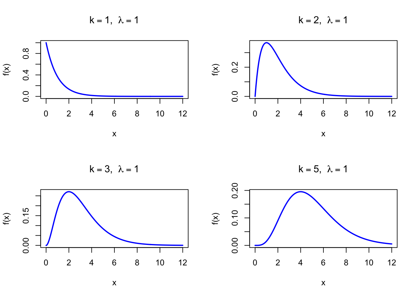
The figure below shows examples of the Erlang Probability Density Function for different shape values with \(\lambda = 1\).

Code
par(mfrow = c(2, 2))
x <- seq(0, 12, length = 500)

plot(x, dgamma(x, shape = 1, rate = 1), type = "l", lwd = 2, col = "blue",
     xlab = "x", ylab = "f(x)", main = expression(paste(k == 1, ",  ", lambda == 1)))

plot(x, dgamma(x, shape = 2, rate = 1), type = "l", lwd = 2, col = "blue",
     xlab = "x", ylab = "f(x)", main = expression(paste(k == 2, ",  ", lambda == 1)))

plot(x, dgamma(x, shape = 3, rate = 1), type = "l", lwd = 2, col = "blue",
     xlab = "x", ylab = "f(x)", main = expression(paste(k == 3, ",  ", lambda == 1)))

plot(x, dgamma(x, shape = 5, rate = 1), type = "l", lwd = 2, col = "blue",
     xlab = "x", ylab = "f(x)", main = expression(paste(k == 5, ",  ", lambda == 1)))

par(mfrow = c(1, 1))
Figure 35.1: Erlang Probability Density Function for various shape values (rate = 1)

35.2 Purpose

The Erlang distribution was developed to model the total waiting time across a fixed number of exponential service stages in telephone switching systems. Its requirement of a positive-integer shape parameter makes it more interpretable than the Gamma distribution in queuing contexts: \(k\) is a literal count of stages. Common applications include:

  • Multi-stage service times in call centers and telecommunications networks
  • Total processing time across sequential stages in manufacturing
  • Aggregate customer service duration when each interaction has \(k\) steps
  • Waiting time before the \(k\)-th arrival in a Poisson process
  • Hypo-exponential distribution building block (sum of different Exponentials)

Relation to the discrete setting. The Erlang distribution is the continuous analog of the Negative Binomial distribution — the Negative Binomial counts discrete failures before the \(k\)-th success; the Erlang measures continuous total time until the \(k\)-th Poisson event.

35.3 Distribution Function

\[ F(x) = 1 - \sum_{n=0}^{k-1}\frac{(\lambda x)^n e^{-\lambda x}}{n!}, \quad x > 0 \]

In R: pgamma(x, shape = k, rate = lambda).

The figure below shows the Erlang Distribution Function for \(k = 3\) and \(\lambda = 1\).

Code
x <- seq(0, 12, length = 500)
plot(x, pgamma(x, shape = 3, rate = 1), type = "l", lwd = 2, col = "blue",
     xlab = "x", ylab = "F(x)", main = "Erlang Distribution Function",
     sub = expression(paste(k == 3, ",  ", lambda == 1)))
Figure 35.2: Erlang Distribution Function (k = 3, rate = 1)

35.4 Moment Generating Function

\[ M_X(t) = \left(\frac{\lambda}{\lambda - t}\right)^k, \quad t < \lambda \]

35.5 1st Uncentered Moment

\[ \mu_1' = \frac{k}{\lambda} \]

35.6 2nd Uncentered Moment

\[ \mu_2' = \frac{k(k+1)}{\lambda^2} \]

35.7 3rd Uncentered Moment

\[ \mu_3' = \frac{k(k+1)(k+2)}{\lambda^3} \]

35.8 4th Uncentered Moment

\[ \mu_4' = \frac{k(k+1)(k+2)(k+3)}{\lambda^4} \]

35.9 2nd Centered Moment

\[ \mu_2 = \frac{k}{\lambda^2} \]

35.10 3rd Centered Moment

\[ \mu_3 = \frac{2k}{\lambda^3} \]

35.11 4th Centered Moment

\[ \mu_4 = \frac{3k(k+2)}{\lambda^4} \]

35.12 Expected Value

\[ \text{E}(X) = \frac{k}{\lambda} \]

35.13 Variance

\[ \text{V}(X) = \frac{k}{\lambda^2} \]

35.14 Median

The median has no closed form and is computed numerically: qgamma(0.5, shape = k, rate = lambda).

35.15 Mode

\[ \text{Mo}(X) = \frac{k-1}{\lambda}, \quad k \geq 1 \]

For \(k = 1\) (Exponential), the mode is 0.

35.16 Coefficient of Skewness

\[ g_1 = \frac{2}{\sqrt{k}} \]

The skewness decreases as \(k\) increases; for large \(k\) the Erlang distribution approaches the Normal distribution.

35.17 Coefficient of Kurtosis

\[ g_2 = 3 + \frac{6}{k} \]

For \(k = 1\) (Exponential), \(g_2 = 9\).

35.18 Parameter Estimation

Since \(k\) must be a positive integer, estimation uses method of moments followed by rounding:

\[ \tilde k = \text{round}\!\left(\frac{\bar x^2}{s^2}\right), \qquad \tilde\lambda = \frac{\tilde k}{\bar x} \]

set.seed(42)
k_true <- 3; lambda_true <- 2
x_obs <- rgamma(100, shape = k_true, rate = lambda_true)

# Method of moments
xbar <- mean(x_obs); s2 <- var(x_obs)
k_hat <- round(xbar^2 / s2)
lambda_hat <- k_hat / xbar
cat("MoM k:     ", k_hat, "\n")
cat("MoM lambda:", round(lambda_hat, 4), "\n")
cat("True k:", k_true, "  True lambda:", lambda_true, "\n")
MoM k:      3 
MoM lambda: 2.0898 
True k: 3   True lambda: 2 

35.19 R Module

35.19.1 RFC

The Erlang Distribution module is available in RFC under the menu “Distributions / Erlang Distribution”.

35.19.2 Direct app link

  • https://shiny.wessa.net/erlang/

35.19.3 R Code

The following code demonstrates Erlang probability calculations using pgamma (which accepts integer shape):

k <- 3; lambda <- 2

# Distribution function: P(X <= x)
pgamma(1.5, shape = k, rate = lambda)

# Quantile (median)
qgamma(0.5, shape = k, rate = lambda)

# Mean and mode
cat("Mean:", k / lambda, "\n")
cat("Mode:", (k - 1) / lambda, "\n")
cat("SD:  ", sqrt(k) / lambda, "\n")

# Generate random Erlang numbers
set.seed(42)
rgamma(10, shape = k, rate = lambda)
[1] 0.5768099
[1] 1.33703
Mean: 1.5 
Mode: 1 
SD:   0.8660254 
 [1] 2.5687787 0.8434274 1.2881428 0.5292550 1.1675090 0.7842371 3.3549583
 [8] 1.2009118 0.5387973 0.3931260

35.20 Example

A call center requires customers to complete \(k = 3\) sequential service stages, each with an independent Exponential service time at rate \(\lambda = 2\) per minute. Total service time \(X \sim \text{Erlang}(3, 2)\) has mean \(k/\lambda = 1.5\) minutes.

k <- 3; lambda <- 2

# P(service time <= 1.5 min)
cat("P(service <= 1.5 min):", pgamma(1.5, shape = k, rate = lambda), "\n")

# Mean, mode, median
cat("Mean (min):", k / lambda, "\n")
cat("Mode (min):", (k - 1) / lambda, "\n")
cat("Median (min):", qgamma(0.5, shape = k, rate = lambda), "\n")
P(service <= 1.5 min): 0.5768099 
Mean (min): 1.5 
Mode (min): 1 
Median (min): 1.33703 
Interactive Shiny app (click to load).
Open in new tab

35.21 Random Number Generator

Erlang random variates are generated as the sum of \(k\) i.i.d. Exponential variates. Using the inverse-CDF form for each:

\[ X = -\frac{1}{\lambda}\ln\!\left(\prod_{i=1}^k U_i\right) = -\frac{1}{\lambda}\sum_{i=1}^k \ln U_i, \quad U_i \overset{\text{i.i.d.}}{\sim} \text{U}(0,1) \]

set.seed(123)
n <- 1000; k <- 3; lambda <- 2

# Sum of k Exponential variates
x_inv <- replicate(n, -sum(log(runif(k))) / lambda)

cat("Simulated mean:", round(mean(x_inv), 4), "\n")
cat("Theoretical mean:", k / lambda, "\n")
cat("Simulated var:", round(var(x_inv), 4), "\n")
cat("Theoretical var:", k / lambda^2, "\n")
Simulated mean: 1.5069 
Theoretical mean: 1.5 
Simulated var: 0.7542 
Theoretical var: 0.75 
Interactive Shiny app (click to load).
Open in new tab

35.22 Property 1: Special Case of Gamma with Integer Shape

The Erlang\((k, \lambda)\) distribution is identical to the Gamma\((k, \lambda)\) distribution when \(k\) is a positive integer. The Gamma distribution allows non-integer shapes (see Chapter 29).

35.23 Property 2: Sum of Independent Exponentials

If \(X_1, \ldots, X_k \overset{\text{i.i.d.}}{\sim} \text{Exp}(\lambda)\) then:

\[ X_1 + \cdots + X_k \sim \text{Erlang}(k, \lambda) \]

This is the defining construction and provides the clearest interpretation: \(X\) is the total time until the \(k\)-th event in a Poisson process.

35.24 Property 3: Special Case \(k = 1\)

When \(k = 1\), the Erlang reduces to the Exponential distribution with rate \(\lambda\):

\[ \text{Erlang}(1, \lambda) = \text{Exp}(\lambda) \]

See Chapter 27.

35.25 Related Distributions 1: Gamma Distribution

The Gamma distribution generalizes the Erlang to non-integer shape parameters (see Chapter 29).

35.26 Related Distributions 2: Exponential Distribution

The Erlang with \(k = 1\) is the Exponential distribution (see Chapter 27).

34  Rayleigh Distribution
36  Logistic Distribution

© 2026 Patrick Wessa. Provided as-is, without warranty.

Feedback: e-mail | Anonymous contributions: click to copy (Sats) | click to copy (XMR)

Cookie Preferences