24  Chi-squared Distribution (2 parameters)

The random variate \(X\) defined for the range \(0 \leq X \leq +\infty\), is said to have a Chi-squared Distribution with 2 parameters (i.e. \(X \sim \chi^2 \left( n, \sigma \right)\)) with shape parameter \(n \in \mathbb{N}^+\) and scale parameter \(\sigma \in \mathbb{R}_0^+\).

This chapter uses a scaled parameterization. If \(Z \sim \chi^2(n)\) (one-parameter form), then \(X=\sigma^2 Z\) follows \(\chi^2(n,\sigma)\) in this notation.

24.1 Probability Density Function

\[ \text{f}(X) = \frac{X^{\frac{n}{2}-1}e^{-\frac{X}{2 \sigma^2}}}{2^{\frac{n}{2}}\Gamma \left[ \frac{n}{2} \right] \sigma^n} \]

24.2 Distribution Function

If \(n/2 \notin \mathbb{N}^+\) then there is no closed form. If \(n/2 \in \mathbb{N}^+\) then

\[ \text{F}(X) = 1 - e^{-\frac{X}{2\sigma^2}}\sum_{j=0}^{r-1}\frac{\left(\frac{X}{2\sigma^2}\right)^j}{j!} \]

where \(r=\frac{n}{2}\).

24.3 Moment Generating Function

\[ \text{M}_X(t) = (1-2\sigma^2t)^{-\frac{n}{2}} \]

where \(t < \frac{1}{2\sigma^2}\).

24.4 Uncentered Moments

\[ \mu_j' = \left(2 \sigma^2\right)^j \frac{\Gamma\left[ \frac{n}{2} +j \right]}{\Gamma \left[ \frac{n}{2} \right]} \]

24.5 Expected Value

\[ \text{E}(X) = n \sigma^2 \]

24.6 Variance

\[ \text{V}(X) = 2 n \sigma^4 \]

24.7 Mode

\[ \text{Mo}(X) = (n-2)\sigma^2 \]

where \(n \geq 2\).

24.8 Skewness

\[ g_1 = 2 \sqrt{\frac{2}{n}} \]

24.9 Kurtosis

\[ g_2 = 3 + \frac{12}{n} \]

24.10 Coefficient of Variation

\[ VC = \sqrt{\frac{2}{n}} \]

24.11 Probability Density Plot

n <- 8
sigma <- 1.5
x <- seq(0, 60, length.out = 1000)
fx <- dchisq(x / sigma^2, df = n) / sigma^2
plot(x, fx, type = "l", col = "steelblue", lwd = 2,
     xlab = "x", ylab = "f(x)",
     main = "Chi-squared density (2 parameters)",
     sub = "(n = 8, sigma = 1.5)")

Figure 24.1: Scaled Chi-squared density (n = 8, sigma = 1.5)

24.12 Random Number Generator

Let

\[ \begin{align*} \begin{cases} \text{U}(0,1) \text{ denote a uniform variate} \\ \text{N}(0,1) \text{ denote a standard normal variate} \\ \text{N}(0,\sigma^2) \text{ denote a normal variate with } \mu = 0 \text{ and variance } \sigma^2 \end{cases} \end{align*} \]

then

\[ \begin{align*} \chi^2(n,\sigma) &\sim - 2 \sigma^2 \ln \left[ \prod_{i=1}^{r} \text{U}_i(0,1) \right] & \text{ } & r=\frac{n}{2} & \text{ (n even)} \\ \chi^2(n,\sigma) &\sim - 2 \sigma^2 \ln \left[ \prod_{i=1}^{r} \text{U}_i(0,1) \right] + \left[ \text{N} \left(0,\sigma^2\right) \right]^2 & \text{ } & r=\frac{n-1}{2} & \text{ (n odd)} \end{align*} \]

24.13 Related Distributions 1: Gamma Representation

The Chi-squared Distribution with parameters \(n\) and \(\sigma\), is a particular form of the Gamma Distribution. Defined in its general form, the probability density function of the three parameter Gamma Distribution is

\[ \text{f}(Y) = \frac{(Y-c)^{a-1}e^{-\frac{Y-c}{b}}}{\Gamma\left[a\right]b^a} \]

with \(c \leq Y \leq +\infty\), \(a > 0\), \(b > 0\), and \(-\infty \leq c \leq +\infty\).

If

\[ \begin{align*} \begin{cases} \text{shape parameter } a = \frac{n}{2} \\ \text{scale parameter } b = 2 \sigma^2 \\ \text{location parameter } c = 0 \end{cases} \end{align*} \]

then the three parameter Gamma Distribution is called a Chi-squared Distribution with parameters \(n\) (degrees of freedom) and \(\sigma\).

24.14 Related Distributions 2: Equivalent Gamma Forms

The Chi-squared variate with parameters \(n\) and \(\sigma\) is equal to the three parameter Gamma variate with location parameter zero, scale parameter \(2\sigma^2\) and shape parameter \(n/2\), or equivalently, is \(2\sigma^2\) times the Gamma variate with location parameter zero, scale parameter one, and shape parameter \(n/2\).

24.15 Related Distributions 3: Sum of Squares of Normal Variables

The Chi-squared variate with parameters \(n\) and \(\sigma\) is equal to the sum of squares of \(n\) independent normal variates with parameters \(\mu = 0\) and variance \(\sigma^2\), i.e.

\[ \chi^2(n,\sigma) \sim \sum_{i=1}^{n} Y_i^2 \]

where \(Y_i = \text{N}(0,\sigma^2)\).

24.16 Related Distributions 4: Noncentral t and F Distributions

The noncentral Chi-squared distribution appears in the construction of both the noncentral \(t\) and noncentral \(F\) distributions. The noncentral \(t\) is formed from the ratio of a Normal with nonzero mean to an independent Chi-squared, while the noncentral \(F\) is the ratio of a noncentral Chi-squared to an independent (central) Chi-squared. These distributions are essential for statistical power analysis (see Chapter 47 and Chapter 48).

24.17 Example

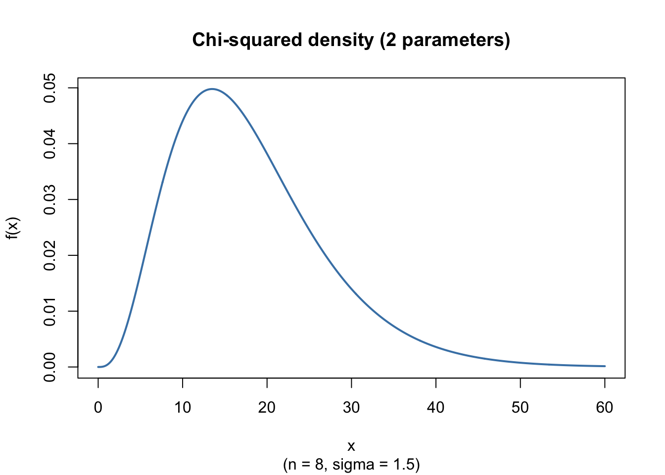
If \(X \sim \chi^2(n=8,\sigma=1.5)\), then:

n <- 8
sigma <- 1.5
px <- pchisq(20 / sigma^2, df = n) # P(X <= 20)
cat("P(X <= 20) =", px, "\n")
cat("E(X) =", n * sigma^2, "\n")
cat("V(X) =", 2 * n * sigma^4, "\n")

P(X <= 20) = 0.6482442 
E(X) = 18 
V(X) = 81 

24.18 Purpose

This scaled form is useful when a Chi-squared structure is present but the measurement scale differs from the unit-scale version. For the standard one-parameter form and additional identities, see Chapter 23.