71 Pearson Correlation

71.1 Definition of Pearson Covariance

\[ \text{C}(xy) = \frac{1}{n} \sum_{i=1}^{n} (x_i - \bar{x}) (y_i - \bar{y}) \]

where

\[ -\infty \leq \text{C}(xy) \leq +\infty \]

\[ \text{V}(x) = s_x^2 = \text{C}(xx) = \frac{1}{n} \sum_{i=1}^{n}(x_i - \bar{x})^2 \]

\[ \text{V}(y) = s_y^2 = \text{C}(yy) = \frac{1}{n} \sum_{i=1}^{n}(y_i - \bar{y})^2 \]

\[ \bar{x} = \frac{1}{n} \sum_{i=1}^{n} x_i \]

and

\[ \bar{y} = \frac{1}{n} \sum_{i=1}^{n} y_i \]

Note: this chapter writes covariance and variance in a population-style form (division by \(n\)). In R, functions such as var, cov, and cor.test use sample estimators with division by \((n-1)\) where relevant. For the correlation coefficient itself, this scaling factor cancels out.

71.2 Definition of Pearson Correlation (Pearson 1895)

\[ r = r_{xy} = \frac{\text{C}(xy)}{\sqrt{\text{V}(x)\text{V}(y)}} = \frac{\text{C}(xy)}{s_x s_y} \]

where

\[ -1 \leq r_{xy} \leq 1 \]

\[ \text{C}(xy) = \frac{1}{n} \sum_{i=1}^{n} (x_i - \bar{x}) (y_i - \bar{y}) \]

\[ -\infty \leq \text{C}(xy) \leq +\infty \]

\[ \text{V}(x) = s_x^2 = \text{C}(xx) = \frac{1}{n} \sum_{i=1}^{n}(x_i - \bar{x})^2 \]

\[ \text{V}(y) = s_y^2 = \text{C}(yy) = \frac{1}{n} \sum_{i=1}^{n}(y_i - \bar{y})^2 \]

\[ \bar{x} = \frac{1}{n} \sum_{i=1}^{n} x_i \]

and

\[ \bar{y} = \frac{1}{n} \sum_{i=1}^{n} y_i \]

71.3 Definition of the Coefficient of Determination

\[ \text{R}^2 = r_{xy}^2 \]

where \(0 \leq \text{R}^2 \leq 1\), \(r = r_{xy} = \frac{\text{C}(xy)}{\sqrt{\text{V}(x)\text{V}(y)}} = \frac{\text{C}(xy)}{s_x s_y}\) and \(-1 \leq r_{xy} \leq 1\).

The Coefficient of Determination can be interpreted as the proportion of the Variance of \(y\) that can be explained by \(x\) (or vice versa).

71.4 t-Test Statistic

\[ t = \frac{r\sqrt{n-2}}{\sqrt{1-r^2}} \sim t_{n-2} \]

where \(r = r_{xy} = \frac{\text{C}(xy)}{\sqrt{\text{V}(x)\text{V}(y)}} = \frac{\text{C}(xy)}{s_x s_y}\) and \(-1 \leq r_{xy} \leq 1\).

Note: under the null hypothesis, the t-Test Statistic is exact when \((x,y)\) follow a bivariate normal distribution. In practice, the test is fairly robust to moderate departures from normality when the sample size is sufficiently large.

71.5 R Module

71.5.1 Public website

The Pearson Correlation module can be found on the public website:

https://compute.wessa.net/corr.wasp

There is also a multivariate R module available which automatically computes correlations for all bivariate combinations:

https://compute.wessa.net/rwasp_pairs.wasp

71.5.2 RFC

The multivariate Pearson Correlation module is available in RFC under the menu item “Descriptive / Multivariate Descriptive Statistics”.

To compute the Pearson Correlation between two quantitative variables in the R console, use the script that is described in Chapter 70.

If you prefer to compute Correlation Matrices on your local machine, the following script can be used in the R console:

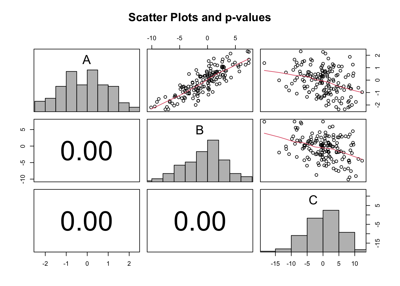
A <- rnorm(150)
B <- A*3 + rnorm(150,0,2)
C <- -2*A + rnorm(150,0,5)
x <- cbind(A, B, C)
#type of correlation (possible values: 'pearson', 'spearman', 'kendall')
par1 = 'pearson'
main = 'Scatter Plots and p-values'
panel.tau <- function(x, y, digits=2, prefix='', cex.cor)
{
  usr <- par('usr'); on.exit(par(usr))
  par(usr = c(0, 1, 0, 1))
  rr <- cor.test(x, y, method=par1)
  r <- round(rr$p.value,2)
  txt <- format(c(r, 0.123456789), digits=digits)[1]
  txt <- paste(prefix, txt, sep='')
  if(missing(cex.cor)) cex <- 0.5/strwidth(txt)
  text(0.5, 0.5, txt, cex = cex)
}
panel.hist <- function(x, ...)
{
  usr <- par('usr'); on.exit(par(usr))
  par(usr = c(usr[1:2], 0, 1.5) )
  h <- hist(x, plot = FALSE)
  breaks <- h$breaks; nB <- length(breaks)
  y <- h$counts; y <- y/max(y)
  rect(breaks[-nB], 0, breaks[-1], y, col='grey', ...)
}
pairs(x,diag.panel=panel.hist, upper.panel=panel.smooth, lower.panel=panel.tau, main=main)

print(paste('Correlations for all pairs of data series (method=',par1,')',sep=''))
n <- ncol(x)
for (i in 1:(n-1)) {
  for (j in (i+1):n) {
    print(paste('Correlation(', colnames(x)[i], ',', colnames(x)[j], ')'))
    print(cor.test(x[,i],x[,j],method=par1))
  }
}

[1] "Correlations for all pairs of data series (method=pearson)"
[1] "Correlation( A , B )"

    Pearson's product-moment correlation

data:  x[, i] and x[, j]
t = 19.02, df = 148, p-value < 2.2e-16
alternative hypothesis: true correlation is not equal to 0
95 percent confidence interval:
 0.7886335 0.8834164
sample estimates:
      cor 
0.8424232 

[1] "Correlation( A , C )"

    Pearson's product-moment correlation

data:  x[, i] and x[, j]
t = -4.3257, df = 148, p-value = 2.783e-05
alternative hypothesis: true correlation is not equal to 0
95 percent confidence interval:
 -0.4700443 -0.1846736
sample estimates:
       cor 
-0.3350199 

[1] "Correlation( B , C )"

    Pearson's product-moment correlation

data:  x[, i] and x[, j]
t = -4.5874, df = 148, p-value = 9.495e-06
alternative hypothesis: true correlation is not equal to 0
95 percent confidence interval:
 -0.4856307 -0.2041089
sample estimates:
       cor 
-0.3528291

To compute the Correlation Matrices, the R code uses the pairs function which is adapted as follows: the diagonal cells contain the Histograms, the cells below the diagonal show the p-value of the correlation test, and the upper diagonal cells display the scatterplots.

71.6 Purpose

Pearson Correlations are used to identify statistical, linear relationships between pairs of variables (with a continuous distribution). In this sense the correlation coefficient is simply a mathematical collinearity measure (i.e. a number which represents to what degree the points of the Scatterplot are on a straight line). If the correlation coefficient is equal to 1 or -1 then it can be concluded that all the points of the Scatterplot lie on exactly one straight line. If the correlation coefficient is close to zero then the points are scattered and do not lie on any straight line.

Note that the Pearson Correlation (just like any other type of correlation) only exists for data that is arranged in wide format with corresponding values in both columns that are examined. For instance, it is impossible to compute the correlation between measurements of females and males.

Even though the Pearson Correlation is mostly used for continuous variables, there is a notable exception in case both variables have binary values. The correlation between two binary variables (i.e. the so-called “Phi coefficient”) is of particular interest within the context of the Confusion Matrix as discussed in Chapter 59 and the Binomial Classification metrics of Chapter 58.

71.7 Phi coefficient (Matthews Correlation)

The Matthews or Phi Correlation coefficient is defined as

\[ \phi = \text{MCC} = \frac{\text{TP} \times \text{TN} - \text{FP} \times \text{FN} }{ \sqrt{(\text{TP}+\text{FP})(\text{TP}+\text{FN})(\text{TN}+\text{FP})(\text{TN}+\text{FN})} } \tag{71.1}\]

which uses the Confusion Matrix in Table 59.2 and can be interpreted like the Pearson Correlation.

If we would reconsider the example from Table 58.1 (which contains two binary variables) then each “Yes” value could be replaced by 1 and each “No” by 0. The result of this transformation is shown in Table 71.1.

Table 71.1: Fraud Predictions of Payment Transactions

Transaction	Is Fraudulent?	Prediction
1	0	1
2	1	1
3	0	0
4	0	0
5	1	0
6	0	0
7	1	0

Based on the values in Table 71.1 it is possible to compute the ordinary Pearson Correlation as is shown in the output below. The Pearson Correlation (\(\simeq 0.09129\)) is computationally equivalent to the Phi Correlation (as was originally developed by Karl Pearson) and is also equal to the Matthews Correlation. Note that the Student t-Test of the Pearson Correlation is not valid for binary data (only the correlation coefficient is).

x = c(0,1,0,0,1,0,1)
y = c(1,1,0,0,0,0,0)
cor(x,y)

[1] 0.09128709

To illustrate the equivalence of the ordinary Pearson Correlation and the Pearson Phi Coefficient, we use the Confusion Matrix from Table 59.1 and apply Equation 71.1 to compute the \(\phi\) value:

\[ \phi = \frac{\text{1} \times \text{3} - \text{1} \times \text{2} }{ \sqrt{(\text{1}+\text{1})(\text{1}+\text{2})(\text{3}+\text{1})(\text{3}+\text{2})} } = \frac{1}{ \sqrt{120} } \simeq 0.09129 \]

The Student t-Test Statistic does not hold for \(\phi\) because binary variables do not have a continuous distribution. Therefore it is better to use the Pearson Chi-Squared Test which is closely related to \(\phi\) and can be tested in various ways (this will be explained in Hypothesis Testing).

71.8 Pros & Cons

71.8.1 Pros

The Pearson Correlation has the following advantages:

it is easy to compute with most statistical software packages (even with spreadsheets)
most readers are familiar with the intuitive concept of correlation
it allows to us to detect linear relationships quickly

71.8.2 Cons

The Pearson Correlation has the following disadvantages:

it is sensitive to outliers
it does not allow us to identify non-linear relationships
hypothesis tests (see Hypothesis Testing) about the Pearson Correlation (which are based on the Student-t distribution) are exact under bivariate normality. For non-normal variables the Student-t test can be used as an approximation, provided the sample is sufficiently large.

71.9 Example with continuous variables

The following analysis, shows the Pearson Correlation between US coffee retail prices and import prices of Arabica coffee from Colombia. The correlation is 0.7 which implies that the variables are highly correlated (the scatter points lie relatively close to a straight line). Since the correlation coefficient is positive, it can be concluded that the slope of the straight line is also positive.

Interactive Shiny app (click to load).

Open in new tab

71.10 Task

Find an example of nonsense correlation (sometimes called spurious correlation) on the Internet. For instance, https://tylervigen.com/spurious-correlations shows many examples of highly correlated relationships which do not make much sense. Try to explain why correlations can be so highly misleading.