91  Variance Reduction Matrix

91.1 Definition

The Variance Reduction Matrix (VRM) is a table which displays the Variance (and the Range) of the time series \(Y_t\) after applying several types of differencing. The exact definitions of these differencing operations is discussed in Introduction to Time Series Analysis but for now it is sufficient to make a distinction between the following situations:

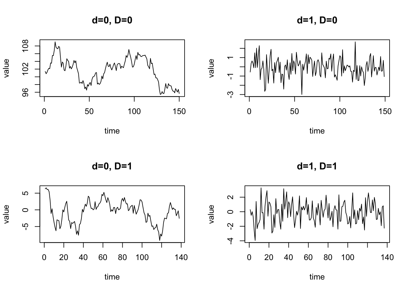
• Differencing with \(d = D = 0\) implies that no transformation is applied at all. In other words, we use the original time series \(Y_t\) without any modification.

• Differencing with \(d = 1\) and \(D = 0\) implies that the long-run trend is removed by applying ordinary differencing: \(Y_t - Y_{t-1}\).

• Differencing with \(d = 0\) and \(D = 1\) implies that the seasonal pattern is reduced by applying seasonal differencing: \(Y_t - Y_{t-s}\) where \(s\) is the seasonality parameter (e.g. \(s = 12\) for monthly time series).

• Differencing with \(d = D = 1\) implies that the long-run trend is removed and the seasonal pattern is reduced by applying the previous two differencing operations in sequence.

There are other forms of differencing as well (these are discussed in Introduction to Time Series Analysis) but these do not occur often in practice.

91.2 Horizontal axis

The horizontal axes of the accompanying Time Plots represent time.

91.3 Vertical axis

The vertical axes of the accompanying Time Plots represent the value of the differenced time series.

91.4 R Module

91.4.1 Public website

The VRM is available on the public website:

• https://compute.wessa.net/rwasp_variancereduction.wasp

91.4.2 RFC

The VRM is also available in RFC under the “Time Series / VRM” menu item.

To compute the Variance Reduction Matrix on your local machine, the following script can be used in the R console:

set.seed(42)
x <- 100 + cumsum(rnorm(150))
summary(x)
par1 <- 12
n.orig <- length(x)
x <- na.omit(x)
n <- length(x)
sx <- sort(x)
for (bigd in 0:2) {
  for (smalld in 0:3) {
    mylabel <- 'V(Y[t],d='
    mylabel <- paste(mylabel,as.character(smalld),sep='')
    mylabel <- paste(mylabel,',D=',sep='')
    mylabel <- paste(mylabel,as.character(bigd),sep='')
    mylabel <- paste(mylabel,') = \t',sep='')
    myx <- x
    if (smalld > 0) myx <- diff(myx,lag=1,differences=smalld)
    if (bigd > 0) myx <- diff(myx,lag=par1,differences=bigd)
    smyx <- sort(myx)
    sn <- length(smyx)
    mylabel <- paste(mylabel, signif(var(myx), digits=6), 
                     '\t\tRange = \t', signif(max(myx)-min(myx), digits=6), 
                     '\t\tTrim Var. = \t', 
                     signif(var(smyx[smyx>quantile(smyx,0.05) & 
                     smyx<quantile(smyx,0.95)]), digits=6), '\n', 
                     sep = '')
    cat(mylabel)
  }
}

op <- par(mfrow=c(2,2))
plot(x,type='l',xlab='time',ylab='value',main='d=0, D=0')
plot(diff(x,lag=1,differences=1),type='l',xlab='time',ylab='value', main='d=1, D=0')
plot(diff(x,lag=par1,differences=1),type='l',xlab='time',ylab='value', main='d=0, D=1')
plot(diff(diff(x,lag=1,differences=1),lag=par1,differences=1),type='l', xlab='time',
     ylab='value',main='d=1, D=1')

par(op)

   Min. 1st Qu.  Median    Mean 3rd Qu.    Max. 
  95.43   98.45  102.22  101.61  103.94  109.06 
V(Y[t],d=0,D=0) =   10.8463     Range =     13.6354     Trim Var. =     7.91626
V(Y[t],d=1,D=0) =   1.00453     Range =     5.69498     Trim Var. =     0.583423
V(Y[t],d=2,D=0) =   1.95202     Range =     7.82459     Trim Var. =     1.14903
V(Y[t],d=3,D=0) =   5.84136     Range =     13.6394     Trim Var. =     3.66059
V(Y[t],d=0,D=1) =   11.1217     Range =     15.7651     Trim Var. =     7.33303
V(Y[t],d=1,D=1) =   2.08126     Range =     7.23604     Trim Var. =     1.40697
V(Y[t],d=2,D=1) =   4.00297     Range =     9.85336     Trim Var. =     2.51814
V(Y[t],d=3,D=1) =   12.0768     Range =     16.5559     Trim Var. =     7.65573
V(Y[t],d=0,D=2) =   22.799      Range =     23.1775     Trim Var. =     13.8154
V(Y[t],d=1,D=2) =   6.17364     Range =     12.8116     Trim Var. =     3.90816
V(Y[t],d=2,D=2) =   11.746      Range =     16.964      Trim Var. =     7.40097
V(Y[t],d=3,D=2) =   35.3822     Range =     26.7309     Trim Var. =     22.4513

To compute the Variance Reduction Matrix, the R code iterates through various combinations of d and D (based on a double loop). For each combination, the script computes the variance, range, and trimmed variance.

91.5 Purpose

The VRM is used to identify whether or not the Variance can be reduced by applying a differencing operation. The parameters \(d\) and \(D\) which correspond to the lowest Variance, often allow us to identify the appropriate differencing operation that is needed to induce stationarity of the time series. The concept of stationarity is mathematically defined at later stages -- the intuitive meaning, however, is simply that the long-run trend and seasonality is removed (or at least strongly reduced).

91.6 Pros & Cons

91.6.1 Pros

The VRM has the following advantages:

• It is easy to compute with a spreadsheet.
• It is easy to understand and often allows us to identify \(d\) and \(D\) very quickly.

91.6.2 Cons

The VRM has the following disadvantages:

• There are not many software packages which feature the VRM.
• Most readers are not familiar with the VRM.
• The VRM is sensitive to outliers. Therefore it is often a good idea to use the trimmed Variance or the Range as alternative measures of Variability.

91.7 Example

Let us consider the Airline Data and apply the VRM analysis. The analysis shows the Variance, Range, and trimmed Variance for a variety of differencing combinations.

Interactive Shiny app (click to load).

Open in new tab

It can be concluded that the lowest (trimmed) Variance is obtained for \(d = D = 1\). This implies that the Airline time series has as long-run trend (\(d=1\)) and a strong seasonal pattern (\(D=1\)).

91.8 Task

Based on the VRM, examine the monthly time series of Marriages and explain the bimodal distribution.