103  Statistical Test of the Population Mean with known Variance

103.1 Theory

103.1.1 Statistical Hypothesis: Testing the Mean with known Variance - Population

The population distribution of the random variable \(X\) is written as \(X \sim \text{N} \left( \mu, \sigma^2 \right)\) where \(\mu\) and \(\sigma^2\) represent the mean and variance of the normal distribution. In this representation it is assumed that \(\mu\) is unknown and \(\sigma^2\) is known.

By introducing the (unrealistic) assumption of a known variance, the mathematical complexity of the statistical hypothesis test is reduced. Hence, this analysis may serve as an initial introduction into hypothesis testing about the mean.

103.1.2 Statistical Hypothesis: Testing the Mean with known Variance - Sample

The statistic for the sample mean is \(\bar{x} = \frac{1}{n} \sum_{i=1}^n x_i\) where \(n\) is the number of observations in the sample. The sample distribution for the mean can be written in terms of the hypotheses \(\text{H}_0\) or \(\text{H}_A\):

\[ \begin{cases}\text{under }\text{H}_0:\ \bar{x} \sim \text{N} \left( \mu_0, \frac{\sigma^2}{n} \right) \\\text{under }\text{H}_A:\ \bar{x} \sim \text{N} \left( \mu_A, \frac{\sigma^2}{n} \right) \end{cases} \]

Observe how the sample mean has a variance which is much smaller than the variance of the original distribution. Under the i.i.d. normality assumption, this is an exact result since \(\mathrm{Var}(\bar{x}) = \sigma^2/n\) (the Central Limit Theorem is not needed here).

103.1.3 Statistical Hypothesis: Testing the Mean with known Variance - Critical Region

Table 103.1: Hypothesis Testing Overview

Null Hypothesis	Alternative Hypothesis	Critical Region
\(\mu \leq \mu_0\)	\(\mu > \mu_0\)	\(\bar{x} \geq \mu_0 + u_{\alpha} \frac{\sigma}{\sqrt{n}}\)
\(\mu \geq \mu_0\)	\(\mu < \mu_0\)	\(\bar{x} \leq \mu_0 - u_{\alpha} \frac{\sigma}{\sqrt{n}}\)
\(\mu = \mu_0\)	\(\mu \neq \mu_0\)	\(\begin{cases} \bar{x} \geq \mu_0 + u_{\frac{\alpha}{2}} \frac{\sigma}{\sqrt{n}} \\ \bar{x} \leq \mu_0 - u_{\frac{\alpha}{2}} \frac{\sigma}{\sqrt{n}} \end{cases}\)

Table 103.2 shows four situations that may occur when applying statistical hypothesis testing. If the Null Hypothesis H\(_0\) is not rejected by the scientist while it is actually true (first column, first row) then the decision of the hypothesis test is correct. We define the probability of this occurrence as \(p = 1 - \alpha\). If the Null Hypothesis H\(_0\) is rejected (while it is, in fact, true) then the scientist’s conclusion is wrong (first column, second row). The probability of this error is defined as \(p = \alpha\) (also called the “type I error”).

If the Null Hypothesis H\(_0\) is not rejected while the Alternative Hypothesis H\(_A\) is true (second column, first row) then a so-called “type II error” is made. The probability of this occurrence is defined as \(p=\beta\). Finally, if the Null Hypothesis H\(_0\) is rejected (i.e. H\(_A\) is supported) while H\(_A\) is actually true (second column, second row) then the scientist’s conclusion is correct. The probability of this happening is \(p = 1 - \beta\).

Table 103.2: Type I and II Errors

Decision	H\(_0\) is true	H\(_A\) is true
Fail to Reject H\(_0\)	Correct (probability \(p = 1 - \alpha\))	Type II Error (probability \(p = \beta\))
Reject H\(_0\)	Type I Error (probability \(p = \alpha\))	Correct (probability \(p = 1 - \beta\))

Table 103.3: Integrals of Type I and II Errors

Decision	H\(_0: \mu \leq \mu_0\)	H\(_A: \mu > \mu_0\)
Fail to Reject H\(_0\)	\(P\left(\bar{x} \leq c \mid H_0: \mu \leq \mu_0\right)=\int_{-\infty}^{c} f(\bar{x})\,d\bar{x}=1-\alpha\), with \(f(\bar{x})\sim N\left(\mu_0,\frac{\sigma^2}{n}\right)\)	\(P\left(\bar{x} \leq c \mid H_A: \mu > \mu_0\right)=\int_{-\infty}^{c} f(\bar{x})\,d\bar{x}=\beta\), with \(f(\bar{x})\sim N\left(\mu_A,\frac{\sigma^2}{n}\right)\)
Reject H\(_0\)	\(P\left(\bar{x} > c \mid H_0: \mu \leq \mu_0\right)=\int_{c}^{\infty} f(\bar{x})\,d\bar{x}=\alpha\), with \(f(\bar{x})\sim N\left(\mu_0,\frac{\sigma^2}{n}\right)\)	\(P\left(\bar{x} > c \mid H_A: \mu > \mu_0\right)=\int_{c}^{\infty} f(\bar{x})\,d\bar{x}=1-\beta\), with \(f(\bar{x})\sim N\left(\mu_A,\frac{\sigma^2}{n}\right)\)

For composite hypotheses such as H\(_0: \mu \leq \mu_0\) versus H\(_A: \mu > \mu_0\), the Type I error rate \(\alpha\) is controlled at the boundary case \(\mu = \mu_0\), whereas the Type II error \(\beta\) is computed for a specific alternative value \(\mu_A\).

Failing to Reject H\(_0\) when it is true

Accepting H\(_0\) when it is true

Failing to Reject H\(_0\) when it is false

Accepting H\(_0\) when it is false

Rejecting H\(_0\) when it is true

Rejecting H\(_0\) when it is true

Rejecting H\(_0\) when it is false

Rejecting H\(_0\) when it is false

103.2 Examples

103.2.1 Statistical Hypothesis: Testing the Mean with known Variance -- Example 1: Critical Value (Region)

103.2.1.1 Problem

Find the critical value c if the following information is available:

• population variance \(\sigma^2 = 0.36\)
• sample size \(n = 9\)
• sample mean \(\bar{x} = 5.35\)
• H\(_0: \mu_0 = 5.2\)
• H\(_A: \mu > \mu_0 = 5.2\) (right-sided test)
• Type I error \(\alpha = 0.05\)

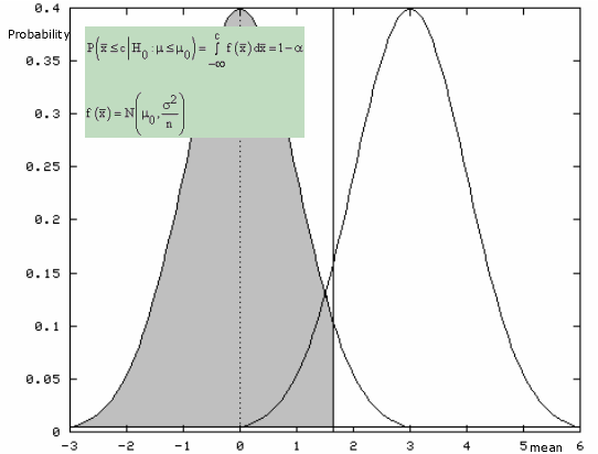
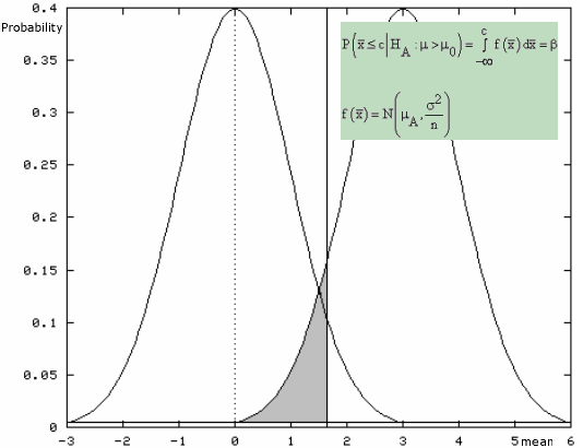
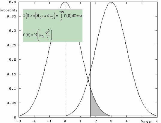
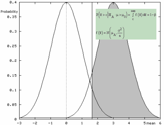
103.2.1.2 Mathematical Solution

\[ \text{P} \left( \bar{x} \geq c \| \text{H}_0: \mu = \mu_0 \right) = \alpha = 0.05 \]

\[ \text{P} \left( \bar{x} \geq c \| \text{H}_0: \mu = \mu_0 \right) = \intop_c^{\infty} \text{f} \left( \bar{x} \| \text{H}_0: \mu = \mu_0 \right) \text{d} \bar{x} = \alpha = 0.05 \]

where

\[ \text{f} \left( \bar{x} \| \text{H}_0: \mu = \mu_0 \right) = \frac{ \sqrt{n} }{ \sigma \sqrt{2 \pi} } e ^ { -\frac{n \left( \bar{x} - \mu_0 \right)^2 }{2 \sigma^2} } = \frac{1}{ \frac{\sigma}{\sqrt{n} } \sqrt{2 \pi} } e ^ { -\frac{ \left( \bar{x} - \mu_0 \right)^2 }{2 \frac{\sigma^2}{n} } } \]

Hence,

\[ \text{P} \left( \bar{x} \geq c \| \text{H}_0: \mu = \mu_0 \right) = \frac{\sqrt{n}}{\sigma \sqrt{2 \pi} } \intop_c^{\infty} e ^ { - \frac{n \left( \bar{x} - \mu_0 \right)^2 }{2 \sigma^2} } \text{d} \bar{x} \]

\[ \text{P} \left( \bar{x} \geq c \| \text{H}_0: \mu = \mu_0 \right) = \frac{1}{ \frac{\sigma}{\sqrt{n}} \sqrt{2 \pi} } \intop_c^{\infty} e ^ { - \frac{ \left( \bar{x} - \mu_0 \right)^2 }{2 \frac{\sigma^2}{n} } } \text{d} \bar{x} = \alpha = 0.05 \]

If we define

\[ u = \frac{ \bar{x} - \mu_0 }{\frac{\sigma}{\sqrt{n} } } \]

then it follows that

\[ u \sim \text{N} \left( 0, 1 \right) \]

\[ \text{P} \left( \frac{\bar{x} - \mu_0 }{\frac{\sigma}{\sqrt{n} } } \geq \frac{c - \mu_0 } {\frac{\sigma } {\sqrt{n} } } \right) = \alpha = 0.05 \]

\[ P\left( u \geq 1.645 \right) = \alpha = 0.05 \]

Hence,

\[ \text{P} \left(u \geq 1.645 \right) = \intop_{1.645}^{\infty} \text{f}(u)\text{d}u = \frac{1 } {\sqrt{2 \pi} } \intop_{1.645}^{\infty} e^{-\frac{u^2 } {2 } } \text{d}u = 0.05 \]

\[ \frac{c - \mu_0 } {\frac{\sigma } {\sqrt{n} } } = 1.645 \]

\[ c = \mu_0 + 1.645 \frac{\sigma } {\sqrt{n} } \]

\[ c = 5.528971 \simeq 5.53 \]

103.2.1.3 Conclusion

The Null Hypothesis H\(_0: \mu_0 = 5.2\) should not be rejected.

103.2.1.4 Software

Interactive Shiny app (click to load).

Open in new tab

The R module can be found on the public website: https://compute.wessa.net/rwasp_hypothesismean1.wasp

To compute this Hypothesis Test on your local machine, the following script can be used in the R console:

par1 = 9 #sample size
par2 = 0.36 #population variance
par3 = 5.35 #sample mean
par4 = 5.2 #null hypothesis about the mean
par5 = 0.05 #type I error
c <- 'NA'
csn <- abs(qnorm(par5))
csn2 <- abs(qnorm(par5/2))
if (par3 == par4) {
  conclusion <- 'Error: the null hypothesis and sample mean must not be equal.'
  conclusion2 <- conclusion
} else {
  cleft <- par4 - csn2 * sqrt(par2) / sqrt(par1)
  cright <- par4 + csn2 * sqrt(par2) / sqrt(par1)
  c2 <- paste('[',cleft)
  c2 <- paste(c2,',')
  c2 <- paste(c2,cright)
  c2 <- paste(c2,']')
  if ((par3 < cleft) | (par3 > cright))
  {
    conclusion2 <- 'Reject the null hypothesis'
  } else {
    conclusion2 <- 'Do not reject the null hypothesis'
  }
}
if (par3 > par4) {
  c <- par4 + csn * sqrt(par2) / sqrt(par1)
  if (par3 < c) {
    conclusion <- 'Do not reject the null hypothesis.'
  } else {
    conclusion <- 'Reject the null hypothesis.'
  }
}
if (par3 < par4) {
  c <- par4 - csn * sqrt(par2) / sqrt(par1)
  if (par3 > c) {
    conclusion <- 'Do not reject the null hypothesis.'
  } else {
    conclusion <- 'Reject the null hypothesis.'
  }
}
print(c)
print(c2)
print(conclusion)

[1] 5.528971
[1] "[ 4.80800720309199 , 5.59199279690801 ]"
[1] "Do not reject the null hypothesis."

103.2.2 Statistical Hypothesis: Testing the Mean with known Variance -- Example 2: P-value (probability)

103.2.2.1 Problem

Compute the p-value if the following information is available:

• population variance \(\sigma^2 = 0.36\)
• sample size \(n = 9\)
• sample mean \(\bar{x} = 5.35\)
• H\(_0: \mu_0 = 5.2\)
• Type I Error \(\alpha = 0.05\)

103.2.2.2 Mathematical Solution

\[ \bar{x} \sim \text{N} \left( \mu, \frac{\sigma^2}{n} \| \text{H}_0: \mu = \mu_0 \right) \]

\[ \frac{\bar{x} - \mu_0 }{\frac{\sigma}{\sqrt{n}}} \sim \text{N}(0,1) \]

\[ \frac{5.35 - 5.2}{\frac{0.6}{\sqrt{9}}} = \frac{0.15}{\frac{0.6}{3}} = 0.75 \]

\[ \text{P}\left( u \geq 0.75 \right) = 0.2266 \]

103.2.2.3 Conclusion

The p-value (= 0.2266) is larger than \(\alpha = 0.05\). Hence, there is no reason to reject H\(_0: \mu_0 = 5.2\)

103.2.2.4 Software

Interactive Shiny app (click to load).

Open in new tab

The R module can be found on the public website:

https://compute.wessa.net/rwasp_hypothesismean2.wasp

To compute this Hypothesis Test on your local machine, the following script can be used in the R console:

par1 = 9 #sample size
par2 = 0.36 #population variance
par3 = 5.35 #sample mean
par4 = 5.2 #null hypothesis about the mean
par5 = 0.05 #type I error
c <- 'NA'
csn <- abs(qnorm(par5))
csn2 <- abs(qnorm(par5/2))
z <- (par3 - par4) / (sqrt(par2/par1))
if (par3 >= par4) {
  p <- 1-pnorm(z)
} else {
  p <- pnorm(z)
}
if (par3 == par4) {
  conclusion <- 'Error: the null hypothesis and sample mean must not be equal.'
  conclusion2 <- conclusion
} else {
  if (p < par5/2) {
    conclusion2 <- 'Reject the null hypothesis'
  } else {
    conclusion2 <- 'Do not reject the null hypothesis'
  }
}
if (p < par5) {
  conclusion <- 'Reject the null hypothesis.'
} else {
  conclusion <- 'Do not reject the null hypothesis.'
}
print(p)
#one and two-sided conclusions
print(conclusion)
print(conclusion2)

[1] 0.2266274
[1] "Do not reject the null hypothesis."
[1] "Do not reject the null hypothesis"

103.2.3 Statistical Hypothesis: Testing the Mean with known Variance -- Example 3: Type II Error

103.2.3.1 Problem

Compute the type II error if the following information is available:

• population variance \(\sigma^2 = 0.36\)
• sample size \(n = 9\)
• sample mean \(\bar{x} = 5.35\)
• H\(_0: \mu_0 = 5.2\)
• Type I Error \(\alpha = 0.05\)
• H\(_A: \mu_A = 5.4\)
• critical value \(c = 5.53\)

103.2.3.2 Mathematical Solution

\[ \text{P} \left( \bar{x} \geq c \| \text{H}_A \right) = 1 - \beta \]

\[ \text{P} \left( \frac{\bar{x} - \mu_A}{\frac{\sigma}{\sqrt{n}}} \geq \frac{c - \mu_A}{\frac{\sigma}{\sqrt{n}}} \right) = 1 - \beta \]

\[ \text{P} \left( u \geq \frac{c - \mu_A}{\frac{\sigma}{\sqrt{n}}} \right) = 1 - \beta \]

\[ \begin{aligned}\frac{c - \mu_A}{\frac{\sigma}{\sqrt{n}}} &= \frac{\mu_0 + 1.645 \frac{\sigma}{\sqrt{n}} - \mu_A}{\frac{\sigma}{\sqrt{n}}} \\ &\simeq \frac{5.528971 - 5.4}{\frac{0.6}{3}} \\ &\simeq 0.644854\end{aligned} \]

\[ \text{P} ( u \geq 0.644854) \simeq 0.2595 \]

\[ \beta \simeq 1 - 0.2595 \simeq 0.74 \]

103.2.3.3 Conclusion

The type II error is 0.74.

103.2.3.4 Software

Interactive Shiny app (click to load).

Open in new tab

The R module can be found on the public website:

https://compute.wessa.net/rwasp_hypothesismean3.wasp

To compute this Hypothesis Test on your local machine, the following script can be used in the R console:

par1 = 9 #sample size
par2 = 0.36 #population variance
par3 = 5.35 #sample mean
par4 = 5.2 #null hypothesis about the mean
par5 = 0.05 #type I error
par6 = 5.4 #alternative hypothesis
c <- 'NA'
csn <- abs(qnorm(par5))
if (par3 == par4) {
  conclusion <- 'Error: the null hypothesis and sample mean must not be equal.'
}
if (par3 > par4) {
  c <- par4 + csn * sqrt(par2) / sqrt(par1)
}
if (par3 < par4) {
  c <- par4 - csn * sqrt(par2) / sqrt(par1)
}
p <- pnorm((c - par6) / (sqrt(par2/par1)))
print(p)

[1] 0.740489

103.2.4 Statistical Hypothesis: Testing the Mean with known Variance -- Example 4: Sample size

103.2.4.1 Problem

Compute the sample size if the following information is available:

• population variance \(\sigma^2 = 0.36\)
• H\(_0: \mu_0 = 5.2\)
• Type I Error \(\alpha = 0.05\)
• H\(_A: \mu_A = 5.4\)
• Type II Error \(\beta = 0.05\)

103.2.4.2 Mathematical Solution 1

\[ \begin{align*} \text{P} \left( \bar{x} \geq c | \text{H}_0 \right) = \alpha = 0.05 \\\text{P} \left( \bar{x} \leq c | \text{H}_A \right) = \beta = 0.05 \end{align*} \]

\[ \begin{align*}\text{P} \left( \frac{\bar{x} - \mu_0}{\frac{\sigma}{\sqrt{n}}} \geq \frac{c - \mu_0}{\frac{\sigma}{\sqrt{n}}} \right) = \alpha = 0.05 \\\text{P} ( u \geq 1.645) = 0.05 \\\frac{c - 5.2}{\frac{\sigma}{\sqrt{n}}} = 1.645\end{align*} \]

\[ \begin{align*}\text{P} \left( \frac{\bar{x} - \mu_A}{\frac{\sigma}{\sqrt{n}}} \leq \frac{c - \mu_A}{\frac{\sigma}{\sqrt{n}}} \right) = \beta = 0.05 \\\text{P} ( u \leq -1.645) = 0.05 \\\frac{c - 5.4}{\frac{\sigma}{\sqrt{n}}} = -1.645\end{align*} \]

\[ \frac{c - 5.2}{c - 5.4} = -1 \Rightarrow c = 5.3 \]

\[ \frac{c - 5.2}{\frac{\sigma}{\sqrt{n}}} = \frac{5.3 - 5.2}{\frac{\sigma}{\sqrt{n}}} = 1.645 \]

\[ 5.3 - 5.2 = 1.645 \frac{\sigma}{\sqrt{n}} \]

\[ \sqrt{n} = \frac{1.645 \cdot 0.6}{0.1} \simeq 9.87 \]

\[ n \simeq 9.87^2 \simeq 97.4169 \Rightarrow n \simeq 98 \]

103.2.4.3 Mathematical Solution 2

\[ \begin{aligned}c &= \mu_0 + u_{\alpha} \frac{\sigma}{\sqrt{n}} &= 5.2 + 1.645 \frac{0.6}{\sqrt{n}} \\c &= \mu_A + u_{1-\beta} \frac{\sigma}{\sqrt{n}} &= 5.4 - 1.645 \frac{0.6}{\sqrt{n}} \\\mu_0 + u_{\alpha} \frac{\sigma}{\sqrt{n}} &= \mu_A + u_{1-\beta} \frac{\sigma}{\sqrt{n}} \\\mu_A - \mu_0 &= u_{\alpha} \frac{\sigma}{\sqrt{n}} - u_{1-\beta} \frac{\sigma}{\sqrt{n}} \\&= \frac{\sigma}{\sqrt{n}} \left( u_{\alpha} - u_{1-\beta} \right)\end{aligned} \]

\[ \begin{aligned}\sqrt{n} &= \frac{\sigma \left( u_{\alpha} - u_{1-\beta} \right)}{\mu_A - \mu_0} \\\sqrt{n} &= \frac{0.6 (1.645 + 1.645)}{5.4 - 5.2} \\&= \frac{0.6 * 3.29}{0.2} = \frac{1.974}{0.2} = 9.87 \\n &= 9.87^2 = 97.4169 \Rightarrow n \simeq 98\end{aligned} \]

103.2.4.4 Conclusion

The sample size is \(n = 98\).

103.2.4.5 Software

Interactive Shiny app (click to load).

Open in new tab

The R module can be found on the public website:

https://compute.wessa.net/rwasp_hypothesismean4.wasp

To compute this Hypothesis Test on your local machine, the following script can be used in the R console:

par1 = 0.36 #Population Variance
par2 = 5.2 #Null Hypothesis about mean
par3 = 5.4 #Alternative Hypothesis about mean
par4 = 0.05 #Type I error (alpha)
par5 = 0.05 #Type II error (beta)
c <- 'NA'
csn <- abs(qnorm(par5))
if (par2 == par3) {
  conclusion <- 'Error: the null hypothesis and alternative hypothesis must not be equal.'
}
ua <- abs(qnorm(par4))
ub <- qnorm(par5)
c <- (par2+ua/ub*(-par3))/(1-(ua/ub))
sqrtn <- ua*sqrt(par1)/(c - par2)
samplesize <- sqrtn * sqrtn
print(ua)
print(ub)
print(c)
print(sqrtn)
print(samplesize)

[1] 1.644854
[1] -1.644854
[1] 5.3
[1] 9.869122
[1] 97.39956

103.2.5 Statistical Hypothesis: Testing the Mean with known Variance -- Example 5: Confidence Intervals for Population Mean

103.2.5.1 Problem

Compute the 95% Confidence Interval for the population mean if the following information is available:

• population variance \(\sigma^2 = 0.36\)
• sample size \(n = 9\)
• sample mean \(\bar{x} = 5.35\)
• probability level under H\(_0\) is 0.95

103.2.5.2 Mathematical Solution for the two-sided confidence interval

\[ \begin{aligned}\text{P} \left( -1.96 \leq \frac{\bar{x} - \mu}{\frac{\sigma}{\sqrt{n}}} \leq 1.96 \right) &= 0.95 \\\text{P} (a \leq \mu \leq b) &= 0.95 \\a &= \bar{x} - 1.96 \frac{\sigma}{\sqrt{n}} = 5.35 - 1.96 \frac{0.6}{3} = 4.958 \\b &= \bar{x} + 1.96 \frac{\sigma}{\sqrt{n}} = 5.35 + 1.96 \frac{0.6}{3} = 5.742\end{aligned} \]

The two-sided 95% confidence interval for the unknown population mean \(\mu\) is \(\bar{x} \pm 0.392\). Hence

\[ \text{95\% confidence interval for } \mu: [4.958, 5.742] \]

103.2.5.3 Mathematical Solution for the right-sided confidence interval

\[ \begin{aligned}\text{P} \left( -1.645 \leq \frac{\bar{x} - \mu}{\frac{\sigma}{\sqrt{n}}} \leq +\infty \right) &= 0.95 \\\text{P}(-\infty \leq \mu \leq b) &= 0.95 \\b &= \bar{x} + 1.645 \frac{\sigma}{\sqrt{n}} = 5.35 + 1.645 \frac{0.6}{3} = 5.679\end{aligned} \]

The right-sided 95% confidence interval for the unknown population mean \(\mu\) is \([ - \infty, 5.679]\). Hence

\[ \text{95\% right-sided confidence interval for } \mu: [-\infty, 5.679] \]

103.2.5.4 Mathematical Solution for the left-sided confidence interval

\[ \begin{aligned}\text{P} \left( -\infty \leq \frac{\bar{x} - \mu}{\frac{\sigma}{\sqrt{n}}} \leq 1.645 \right) &= 0.95 \\\text{P}(a \leq \mu \leq +\infty) &= 0.95 \\a &= \bar{x} - 1.645 \frac{\sigma}{\sqrt{n}} = 5.35 - 1.645 \frac{0.6}{3} = 5.021\end{aligned} \]

The left-sided 95% confidence interval for the unknown population mean \(\mu\) is \([ 5.021, +\infty]\). Hence

\[ \text{95\% left-sided confidence interval for } \mu: [5.021, +\infty] \]

103.2.5.5 Conclusion

The two-sided 95% confidence interval for \(\mu\) is \([4.958, 5.742]\). The right one-sided 95% confidence interval is \([-\infty, 5.679]\) whereas the left one-sided interval is \([5.021, \infty)\). In repeated sampling, these procedures achieve 95% coverage.

103.2.5.6 Software

Interactive Shiny app (click to load).

Open in new tab

The R module can be found on the public website:

https://compute.wessa.net/rwasp_hypothesismean5.wasp

To compute this Hypothesis Test on your local machine, the following script can be used in the R console:

par1 = 0.36 #Population Variance
par2 = 9 #Sample Size
par3 = 5.35 #Sample Mean
par4 = 0.95 #Confidence Interval
sigma <- sqrt(par1)
sqrtn <- sqrt(par2)
ua <- par3 - abs(qnorm((1-par4)/2))* sigma / sqrtn
ub <- par3 + abs(qnorm((1-par4)/2))* sigma / sqrtn
print(ua)
print(ub)
ul <- par3 - qnorm(par4) * sigma / sqrtn
print(ul)
ur <- par3 + qnorm(par4) * sigma / sqrtn
print(ur)

[1] 4.958007
[1] 5.741993
[1] 5.021029
[1] 5.678971

103.2.6 Statistical Hypothesis: Testing the Mean with known Variance -- Example 6: Acceptance Regions for Sample Mean (under H\(_0\))

103.2.6.1 Problem

Compute the 95% acceptance region (under H\(_0\)) for the sample mean if the following information is available:

• population variance \(\sigma^2 = 0.36\)
• sample size \(n = 9\)
• \(H_0: \mu_0 = 5.2\)
• probability level under H\(_0\) is 0.95

103.2.6.2 Mathematical Solution for the two-sided acceptance region

\[ \begin{aligned}\text{P} \left( -1.96 \leq \frac{\bar{x} - \mu_0}{\frac{\sigma}{\sqrt{n}}} \leq 1.96 \right) &= 0.95 \\\text{P} (a \leq \bar{x} \leq b) &= 0.95 \\a &= \mu_0 - 1.96 \frac{\sigma}{\sqrt{n}} = 5.2 - 1.96 \frac{0.6}{3} = 4.808 \\b &= \mu_0 + 1.96 \frac{\sigma}{\sqrt{n}} = 5.2 + 1.96 \frac{0.6}{3} = 5.592\end{aligned} \]

The two-sided 95% acceptance region for the sample mean \(\bar{x}\) (under H\(_0\)) is \(\mu_0 \pm 0.392\). Hence

\[ \text{P} (4.808 \leq \bar{x} \leq 5.592) = 0.95 \]

103.2.6.3 Mathematical Solution for the right-sided acceptance region

\[ \begin{aligned}\text{P} \left( -\infty \leq \frac{\bar{x} - \mu_0}{\frac{\sigma}{\sqrt{n}}} \leq 1.645 \right) &= 0.95 \\\text{P}(-\infty \leq \bar{x} \leq b) &= 0.95 \\b &= \mu_0 + 1.645 \frac{\sigma}{\sqrt{n}} = 5.2 + 1.645 \frac{0.6}{3} = 5.529\end{aligned} \]

The right-sided 95% acceptance region for the sample mean \(\bar{x}\) (under H\(_0\)) is \([ - \infty, 5.529]\). Hence

\[ \text{P} ( - \infty \leq \bar{x} \leq 5.529) = 0.95 \]

103.2.6.4 Mathematical Solution for the left-sided acceptance region

\[ \begin{aligned}\text{P} \left( -1.645 \leq \frac{\bar{x} - \mu_0}{\frac{\sigma}{\sqrt{n}}} \leq +\infty \right) &= 0.95 \\\text{P}(a \leq \bar{x} \leq +\infty) &= 0.95 \\a &= \mu_0 - 1.645 \frac{\sigma}{\sqrt{n}} = 5.2 - 1.645 \frac{0.6}{3} = 4.871\end{aligned} \]

The left-sided 95% acceptance region for the sample mean \(\bar{x}\) (under H\(_0\)) is \([ 4.871, +\infty]\). Hence

\[ \text{P} ( 4.871 \leq \bar{x} \leq +\infty) = 0.95 \]

103.2.6.5 Conclusion

The two-sided acceptance region can be written as P\(\left( 4.808 \leq \bar{x} \leq 5.592 \right) = 0.95\). The right one-sided acceptance region is P\(\left( -\infty \leq \bar{x} \leq 5.529 \right) = 0.95\) whereas the left one-sided acceptance region can be written as P\(\left( 4.871 \leq \bar{x} \leq \infty \right) = 0.95\).

103.2.6.6 Software

Interactive Shiny app (click to load).

Open in new tab

The R module can be found on the public website:

https://compute.wessa.net/rwasp_hypothesismean6.wasp

To compute this Hypothesis Test on your local machine, the following script can be used in the R console:

par1 = 0.36 #Population Variance
par2 = 9 #Sample Size
par3 = 5.2 #Null Hypothesis
par4 = 0.95 #Confidence Interval
sigma <- sqrt(par1)
sqrtn <- sqrt(par2)
ua <- par3 - abs(qnorm((1-par4)/2))* sigma / sqrtn
ub <- par3 + abs(qnorm((1-par4)/2))* sigma / sqrtn
print(ua)
print(ub)
ul <- par3 - qnorm(par4) * sigma / sqrtn
print(ul)
ur <- par3 + qnorm(par4) * sigma / sqrtn
print(ur)

[1] 4.808007
[1] 5.591993
[1] 4.871029
[1] 5.528971