A model that fits its training data well is not necessarily a model that will work well on new data. Model validation is the set of procedures used to estimate how a fitted model will perform on observations it has not seen. This chapter introduces the main validation strategies used throughout this part and in the Guided Model Building app.
160.1 Overfitting and the Need for Held-Out Data
Overfitting occurs when a model captures noise in the training data rather than the underlying pattern. A model that is too flexible will fit the training data almost perfectly but generalize poorly.
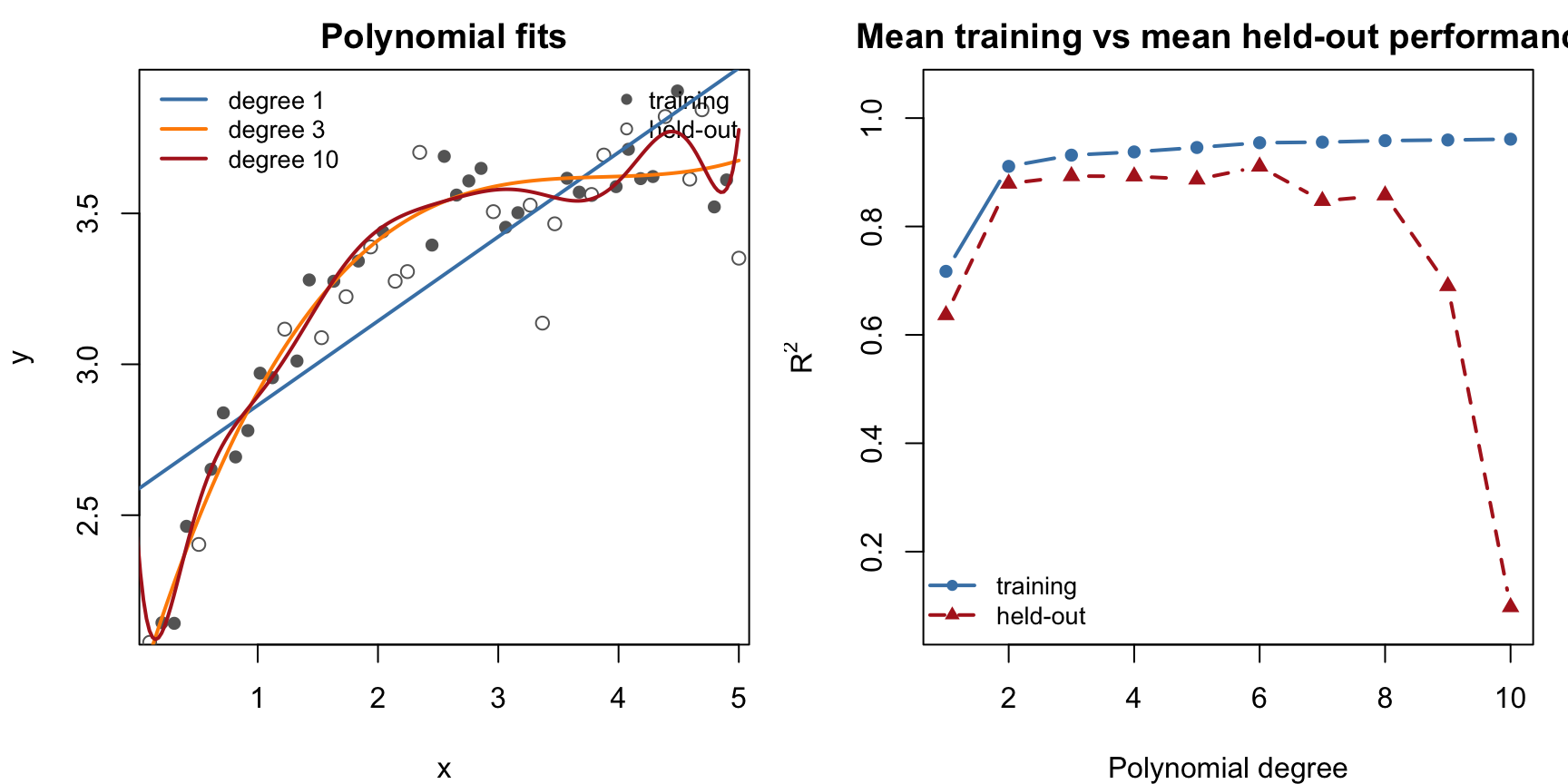
The following example makes this concrete. A small synthetic dataset is fitted with polynomials of increasing degree. As the degree increases, the training fit improves. To keep the held-out pattern readable for teaching purposes, the right-hand panel averages the training and held-out \(R^2\) values across many random splits of the same dataset rather than relying on a single noisy split.
Overfitting illustrated with polynomial regression. Left: fitted curves at degree 1, 3, and 10 for one illustrative split. Right: mean training and mean held-out R-squared across many random splits of the same dataset.
The left panel shows that the degree-10 polynomial follows much more of the local variation than the lower-degree fits. The right panel shows that the mean held-out \(R^2\) drops once model flexibility becomes excessive, even though mean training \(R^2\) continues to rise. The point where the two lines diverge is where overfitting begins.
This is why validation requires held-out data: performance on the training set alone cannot tell you whether the model has learned the pattern or memorized the noise.
160.2 Single Holdout Split
The simplest validation method splits the data once into a training set and a test set. The model is fitted on the training set and evaluated on the test set. This is exactly what the training percentage slider in the app available in the menu Models / Manual Model Building does (see Section 159.7).
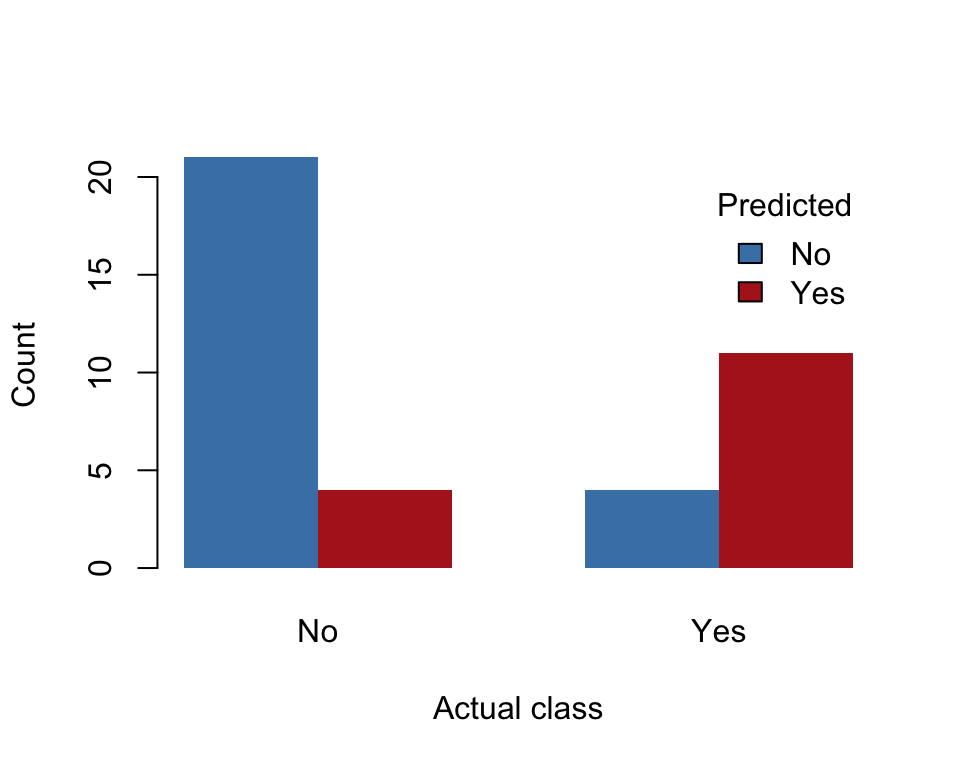
Confusion matrix from a single holdout split of Pima.tr at 80% training
The single holdout split has a limitation: its result depends on which rows happen to fall into the training set and which fall into the test set. A different random split can produce a noticeably different accuracy estimate.
160.3 Repeated Holdout
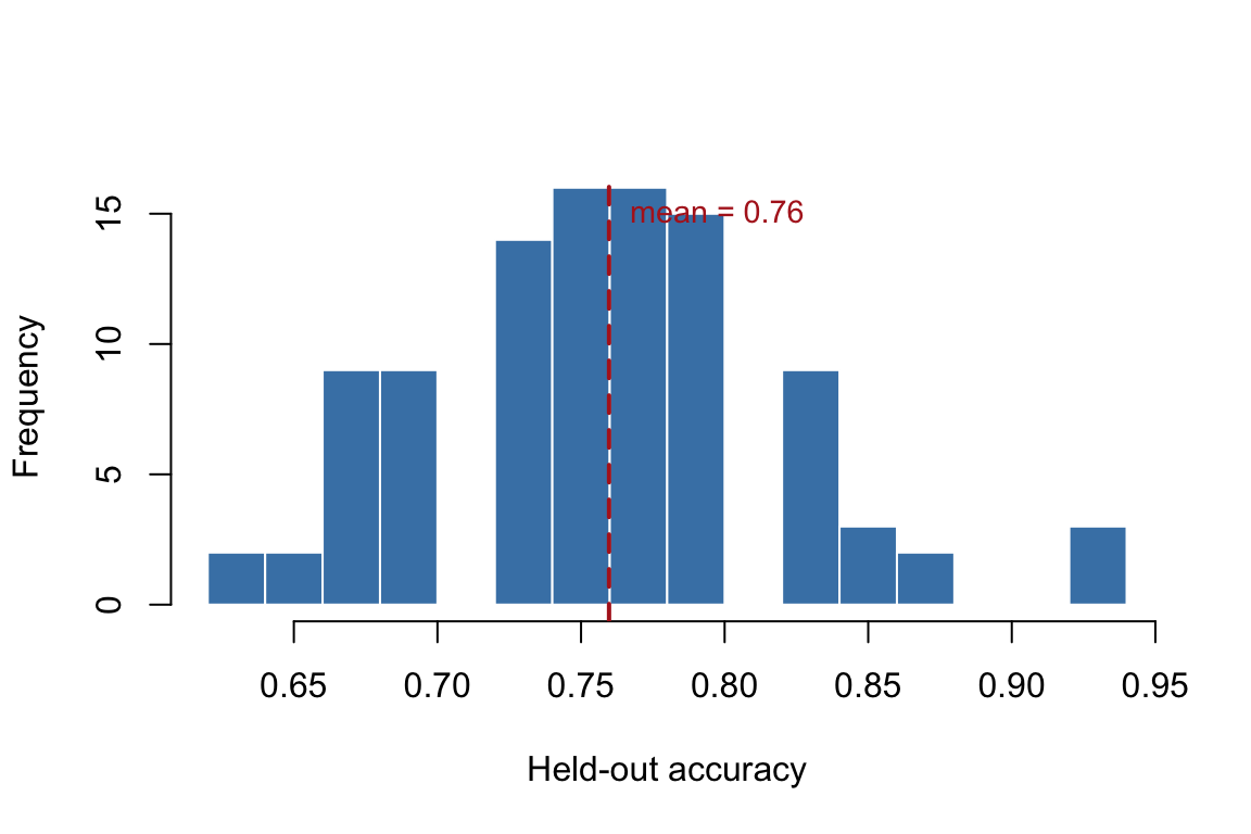
Repeated holdout addresses the instability of a single split by repeating the procedure many times. Each repetition uses a fresh random split, fits the model, and records the held-out performance. The final estimate is the average across repetitions.
Distribution of held-out accuracy across 100 repeated holdout splits
The histogram shows that individual splits produce accuracy values that scatter over a noticeable range. The dashed line marks the average. This average is a more reliable estimate than any single split because it absorbs the randomness of the split itself.
The Guided Model Building app uses repeated holdout as its default validation strategy for tabular data (see Section 163.4.4 and Section 163.5.2).
160.4 Stratified Holdout
Random holdout splits do not guarantee that the class proportions in the training and test sets match the population proportions. When the target is unbalanced — as in the Pima dataset, where about two thirds of cases are negative — a random split can occasionally produce a test set with a substantially different class distribution.
Stratified holdout solves this by splitting within each class separately, so the proportions are preserved by construction.
Positive-class share across 20 random splits (left) versus 20 stratified splits (right). The dashed line marks the true share.
The random splits show visible wobble in the positive-class share. The stratified splits cluster tightly around the true proportion (dashed line). When the dataset is small or the class balance is uneven, stratification prevents accidental evaluation on an unrepresentative test set.
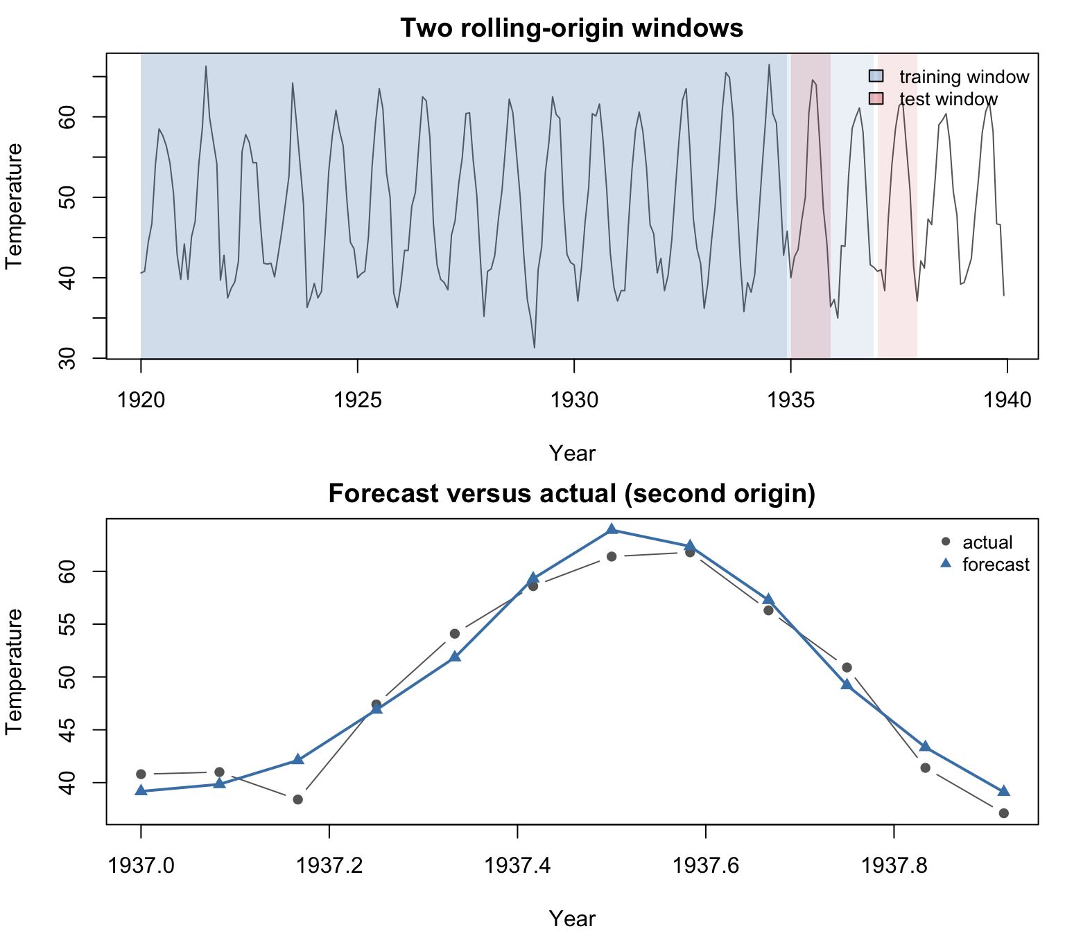
160.5 Rolling-Origin Validation for Time Series
When the data are ordered in time, random holdout splits are not appropriate because they ignore temporal dependence. A model should not be evaluated on observations that precede the training period.
Rolling-origin validation respects the time ordering. The procedure is:
train the model on all observations up to a cutoff point,
forecast the next \(h\) observations,
record the forecast error,
advance the cutoff by one period and repeat.
The error metrics are averaged across all origins to produce a stable summary.
Registered S3 method overwritten by 'quantmod':
  method            from
  as.zoo.data.frame zoo
fc <- forecast::forecast(arima_fit, h = h)actual_vals <- nottem_vals[(origin_2 +1):min(origin_2 + h, n_obs)]fc_time <- nottem_time[(origin_2 +1):min(origin_2 + h, n_obs)]plot(fc_time, actual_vals, type ="b", pch =16, col ="grey40",xlab ="Year", ylab ="Temperature",ylim =range(c(actual_vals, as.numeric(fc$mean)), na.rm =TRUE),main ="Forecast versus actual (second origin)")lines(fc_time, as.numeric(fc$mean)[seq_along(fc_time)],col ="steelblue", lwd =2)points(fc_time, as.numeric(fc$mean)[seq_along(fc_time)],pch =17, col ="steelblue")legend("topright", pch =c(16, 17), col =c("grey40", "steelblue"),legend =c("actual", "forecast"), bty ="n", cex =0.85)
Rolling-origin validation on the nottem series. Top: two training windows (blue) and their corresponding test windows (red). Bottom: forecast versus actual for the second origin.
The top panel shows how the training window grows as the origin advances. The bottom panel shows the forecast produced at the second origin against the actual values. The Guided Model Building app uses rolling-origin validation for all time-series models (see Section 164.4.1 and Chapter 153).
160.6 Comparison Metrics for Regression and Classification
Validation produces held-out predictions. To compare models, those predictions must be summarized into metrics. The appropriate metrics depend on whether the target is continuous (regression) or categorical (classification).
160.6.1 Regression Metrics
Metric
Definition
Interpretation
RMSE
\(\sqrt{\frac{1}{n}\sum (y_i - \hat{y}_i)^2}\)
average error magnitude, penalizes large errors more
MAE
\(\frac{1}{n}\sum |y_i - \hat{y}_i|\)
average absolute error, less sensitive to outliers
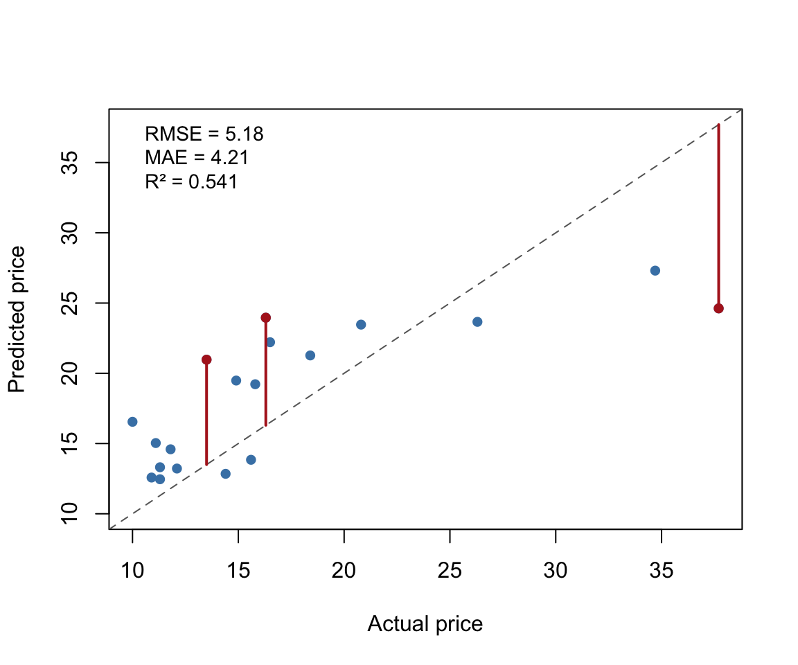
Predicted versus actual price for Cars93. Segments mark the three largest residuals.
The three red segments connect the largest prediction errors to the diagonal. These are the observations that contribute most to the RMSE. If the squared penalty matters (as it does in RMSE), the model’s performance is substantially driven by its worst predictions.
F1 is the harmonic mean of precision and sensitivity. Precision is the share of predicted positives that are truly positive. The harmonic mean ensures that F1 is low whenever either precision or sensitivity is low.
MCC (Matthews correlation coefficient) is a correlation coefficient between the observed and predicted binary classifications. It takes values between \(-1\) and \(+1\), where \(+1\) indicates perfect prediction, \(0\) indicates no better than random, and \(-1\) indicates total disagreement. Unlike accuracy, MCC remains informative when the classes are unbalanced.
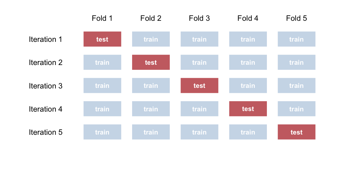
160.7 k-Fold Cross-Validation
In k-fold cross-validation, the data are divided into \(k\) equally sized groups (folds). The model is trained on \(k - 1\) folds and evaluated on the remaining fold. This is repeated \(k\) times so that every observation serves as a test case exactly once. The final metric is the average across folds.
par(mar =c(2, 6, 2, 1))k <-5plot(NULL, xlim =c(0.5, k +0.5), ylim =c(0.5, k +0.5),xlab ="", ylab ="", xaxt ="n", yaxt ="n", bty ="n",main ="")for (i in1:k) {for (j in1:k) { col <-if (j == i) "firebrick"else"steelblue" alpha <-if (j == i) 0.7else0.3rect(j -0.4, k - i +1-0.35, j +0.4, k - i +1+0.35,col =adjustcolor(col, alpha.f = alpha), border ="white", lwd =2) label <-if (j == i) "test"else"train"text(j, k - i +1, label, cex =0.7, col ="white", font =2) }mtext(paste("Iteration", i), side =2, at = k - i +1, las =1, cex =0.8, line =0.5)}mtext(paste("Fold", 1:k), side =3, at =1:k, cex =0.8)
Schematic of 5-fold cross-validation. Each row is one iteration. The shaded block is the test fold.
This handbook uses repeated holdout rather than k-fold cross-validation as the primary validation method. The reason is practical: repeated holdout maps directly to the training percentage slider in the app available in the menu Models / Manual Model Building and to the repeated-holdout validation used by the Guided Model Building app. The two methods address the same fundamental problem — estimating held-out performance — but repeated holdout is easier to connect to the tools used throughout the book.
k-fold cross-validation is widely used in practice and has the advantage that every observation appears in the test set exactly once. It is especially useful when the dataset is small and wasting observations on a large held-out set is costly.
160.8 Practical Exercises
Run the overfitting example above with a different set.seed value. Does the crossover point between training and held-out \(R^2\) always occur at the same polynomial degree?
Change the number of repetitions in the repeated holdout example from 100 to 10. How does the histogram change? How does the mean change?
Modify the stratified holdout example to use a 60/40 split instead of 80/20. Does the difference between random and stratified splits become larger or smaller?
In the rolling-origin example, change the forecast horizon from 12 to 24. How does this affect the forecast accuracy?
Compute the RMSE and MAE for the Cars93 regression example. Which metric is more affected by the three largest residuals?
Explain in your own words why k-fold cross-validation guarantees that every observation is tested exactly once, whereas repeated holdout does not.