The Gamma distribution answers the question: how long until the \(k\)-th event? It generalizes the Exponential distribution — which covers the waiting time for a single event — to model the accumulated waiting time across multiple events, and provides a flexible family for any positive continuous measurement where right-skewness needs to be controlled.
Formally, the random variate \(X\) defined for the range \(X > 0\), is said to have a Gamma Distribution (i.e. \(X \sim \text{Gamma}(k, \lambda)\)) with shape parameter \(k > 0\) and rate parameter \(\lambda > 0\).
The Gamma distribution generalizes the Exponential distribution (shape \(k = 1\)) and the Erlang distribution (integer shape), and is related to the Chi-squared distribution. In R, the shape parameter is shape and the rate parameter is rate; the equivalent scale parameterization \(\theta = 1/\lambda\) is also accepted — pass scale\(= 1/\lambda\) as an argument instead of rate.
where \(\Gamma(k) = \int_0^\infty t^{k-1} e^{-t}\, dt\) is the Gamma function. For positive integers \(k\), \(\Gamma(k) = (k-1)!\).
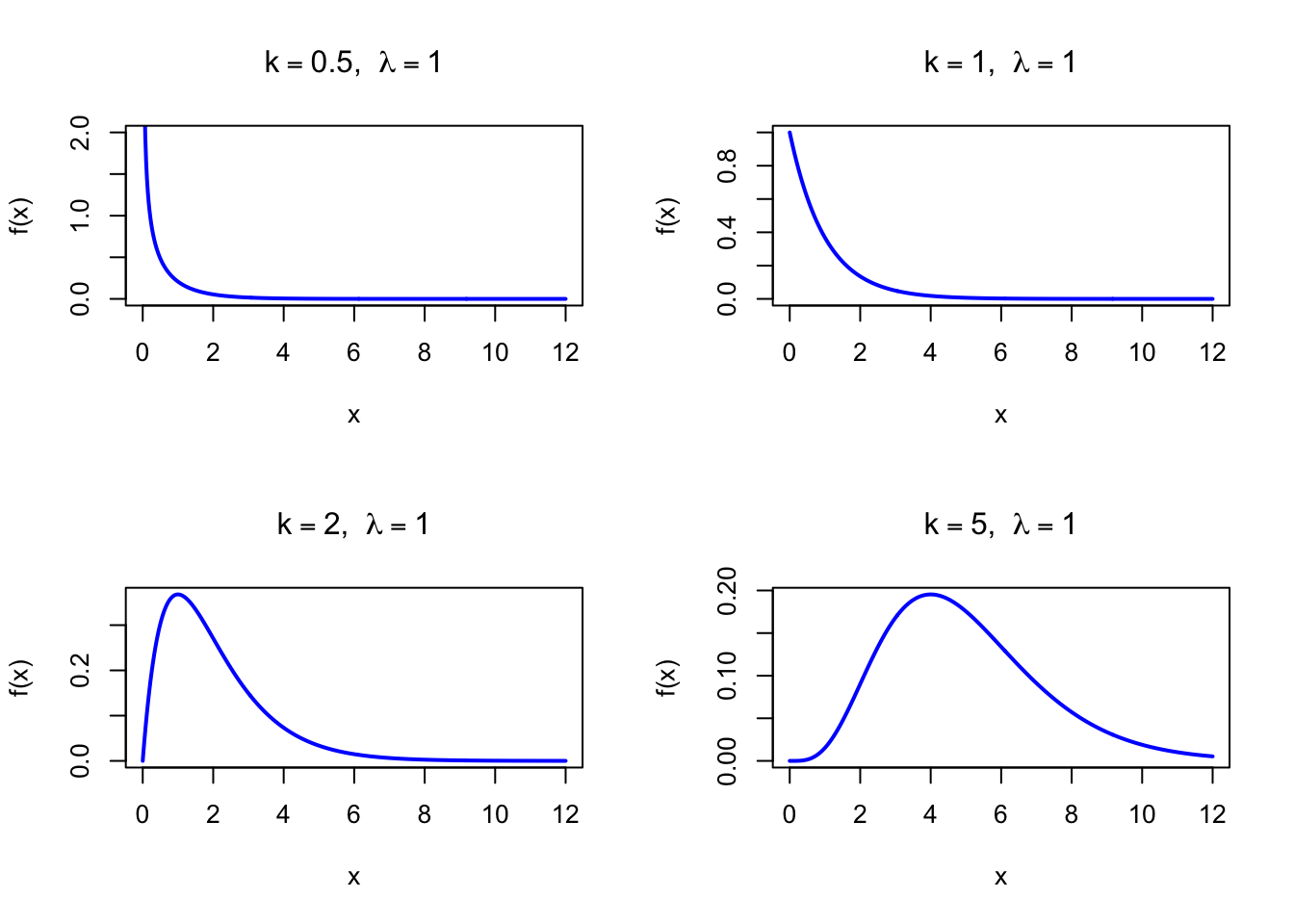
The figure below shows examples of the Gamma Probability Density Function for different shape values with \(\lambda = 1\).
Code
par(mfrow =c(2, 2))x <-seq(0, 12, length =500)plot(x, dgamma(x, shape =0.5, rate =1), type ="l", lwd =2, col ="blue",xlab ="x", ylab ="f(x)", main =expression(paste(k ==0.5, ", ", lambda ==1)),ylim =c(0, 2))plot(x, dgamma(x, shape =1, rate =1), type ="l", lwd =2, col ="blue",xlab ="x", ylab ="f(x)", main =expression(paste(k ==1, ", ", lambda ==1)))plot(x, dgamma(x, shape =2, rate =1), type ="l", lwd =2, col ="blue",xlab ="x", ylab ="f(x)", main =expression(paste(k ==2, ", ", lambda ==1)))plot(x, dgamma(x, shape =5, rate =1), type ="l", lwd =2, col ="blue",xlab ="x", ylab ="f(x)", main =expression(paste(k ==5, ", ", lambda ==1)))par(mfrow =c(1, 1))
Figure 29.1: Gamma Probability Density Function for various shape values (rate = 1)
29.2 Purpose
The Gamma distribution models the total waiting time until the \(k\)-th event in a process where individual waiting times are independent and exponentially distributed. Its shape parameter \(k\) controls the degree of skewness, making it a flexible family for any positive continuous measurement. Common applications include:
Waiting time until the \(k\)-th customer arrival, failure, or detected signal
Aggregate insurance claims and total loss amounts
Rainfall amounts, flood volumes, and similar hydrology measurements
Processing and repair times in operations research and reliability
Prior distribution for rate and precision parameters in Bayesian models
Relation to the discrete setting. The Gamma\((k, \lambda)\) distribution is the continuous analog of the Negative Binomial distribution. The Negative Binomial counts the total number of discrete trials until the \(k\)-th success; the Gamma measures the continuous total waiting time until the \(k\)-th event in a Poisson process. When the shape \(k\) is a positive integer, this analogy is exact via the sum-of-Exponentials construction: just as a Negative Binomial count is the sum of \(k\) i.i.d. Geometric variates, a Gamma\((k,\lambda)\) variate is the sum of \(k\) i.i.d. Exp\((\lambda)\) variates.
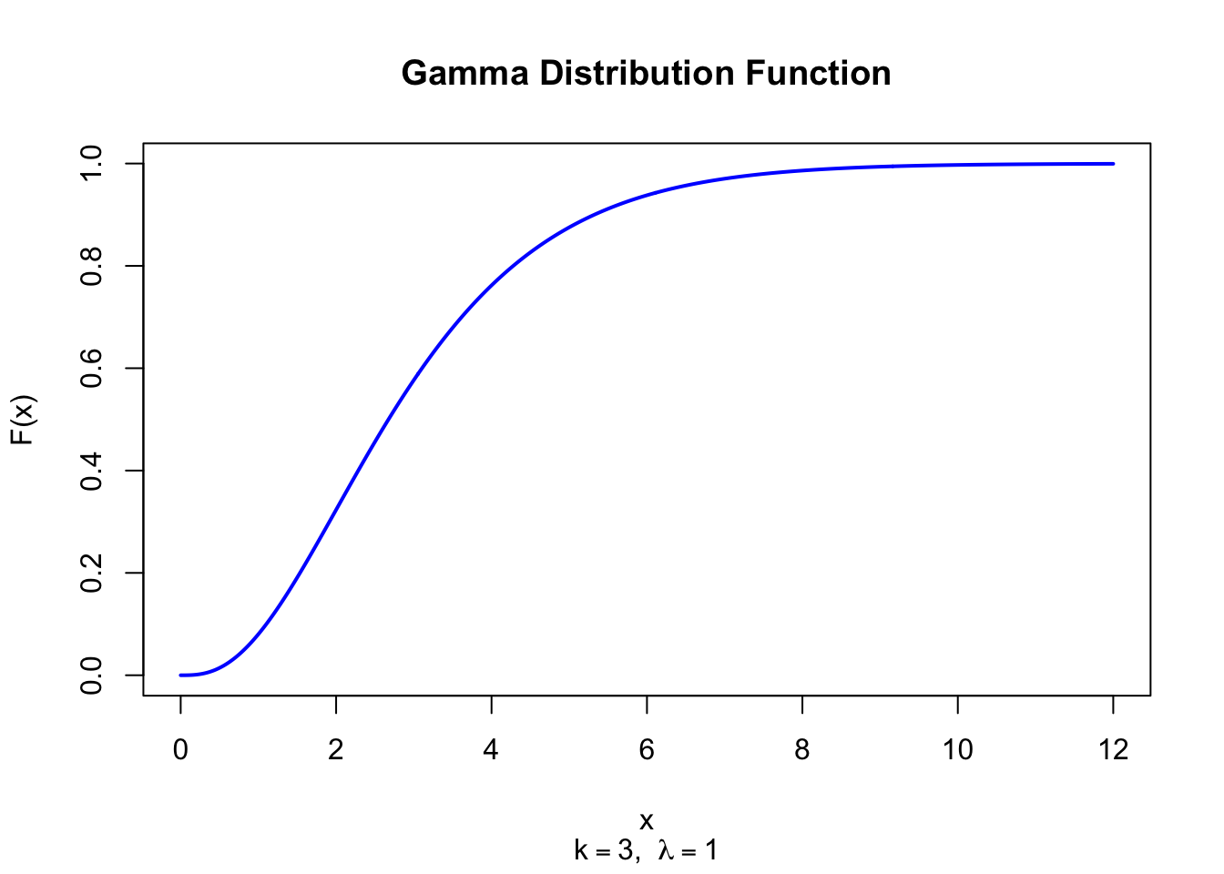
where \(\gamma(k, z) = \int_0^z t^{k-1} e^{-t}\, dt\) is the lower incomplete gamma function. The ratio \(\gamma(k, z)/\Gamma(k)\) is also called the regularized incomplete gamma function and is computed by pgamma() in R.
The figure below shows the Gamma Distribution Function for \(k = 3\) and \(\lambda = 1\).
Code
x <-seq(0, 12, length =500)plot(x, pgamma(x, shape =3, rate =1), type ="l", lwd =2, col ="blue",xlab ="x", ylab ="F(x)", main ="Gamma Distribution Function",sub =expression(paste(k ==3, ", ", lambda ==1)))
Figure 29.2: Gamma Distribution Function (shape = 3, rate = 1)
For \(0 < k < 1\), the density is strictly decreasing on \((0, \infty)\) and the mode is at the left boundary (\(x \to 0^+\)). For \(k = 1\), the mode coincides with the left boundary at 0 (Exponential distribution).
29.16 Coefficient of Skewness
\[
g_1 = \frac{2}{\sqrt{k}}
\]
The Gamma distribution is always right-skewed. Skewness decreases as the shape parameter \(k\) increases, and the distribution approaches symmetry (and normality, by the CLT) as \(k \to \infty\).
29.17 Coefficient of Kurtosis
\[
g_2 = 3 + \frac{6}{k}
\]
The excess kurtosis is \(6/k\), which is always positive, indicating heavier tails than the Normal distribution. As \(k \to \infty\), the kurtosis approaches 3 (Normal).
29.18 Parameter Estimation
The maximum likelihood estimators of \(k\) and \(\lambda\) do not have closed-form solutions. A method-of-moments starting point gives \(\tilde{k} = \bar{x}^2/s^2\) and \(\tilde{\lambda} = \bar{x}/s^2\), where \(s^2\) is the sample variance. The fitdistr function in R’s MASS package uses these as starting values for numerical optimization.
A service counter has customers arriving according to a Poisson process at rate \(\lambda = 0.5\) arrivals per minute. The waiting time until the 3rd customer arrives follows \(X \sim \text{Gamma}(3, 0.5)\), with mean \(3/0.5 = 6\) minutes and standard deviation \(\sqrt{3}/0.5 \approx 3.46\) minutes.
k <-3lambda <-0.5# P(X <= 8): probability the 3rd customer arrives within 8 minutescat("P(3rd arrival within 8 min):", round(pgamma(8, shape = k, rate = lambda), 4), "\n")# P(X > 10): probability of waiting more than 10 minutescat("P(wait > 10 min):", round(1-pgamma(10, shape = k, rate = lambda), 4), "\n")# 95th percentile: 95% of the time the 3rd customer arrives before this timecat("95th percentile (min):", round(qgamma(0.95, shape = k, rate = lambda), 2), "\n")
A Gamma\((k, \lambda)\) variate with integer shape \(k\) can be generated as the sum of \(k\) independent Exp\((\lambda)\) variates (see Property 1 below). For non-integer \(k\), R uses Marsaglia and Tsang’s efficient acceptance-rejection algorithm.
set.seed(123)n <-1000k <-3lambda <-0.5# Sum-of-exponentials method (integer k only)x_sum <-rowSums(matrix(rexp(n * k, rate = lambda), nrow = n))# Built-in functionx_rgamma <-rgamma(n, shape = k, rate = lambda)cat("Sum-of-Exp: mean =", round(mean(x_sum), 4)," var =", round(var(x_sum), 4), "\n")cat("rgamma(): mean =", round(mean(x_rgamma), 4)," var =", round(var(x_rgamma), 4), "\n")cat("Theoretical: mean =", k/lambda," var =", k/lambda^2, "\n")
Sum-of-Exp: mean = 6.0951   var = 13.319
rgamma():   mean = 5.9367   var = 10.9331
Theoretical: mean = 6   var = 12
Code
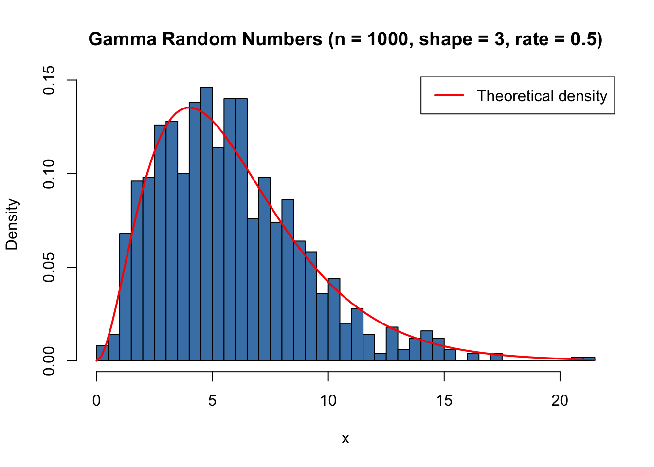
set.seed(123)x <-rgamma(1000, shape =3, rate =0.5)hist(x, breaks =35, col ="steelblue", freq =FALSE,xlab ="x", main ="Gamma Random Numbers (n = 1000, shape = 3, rate = 0.5)")curve(dgamma(x, shape =3, rate =0.5), add =TRUE, col ="red", lwd =2)legend("topright", legend ="Theoretical density", col ="red", lwd =2)
Figure 29.3: Histogram of simulated Gamma random numbers (n = 1000, shape = 3, rate = 0.5)
29.27 Related Distributions 3: Waiting Time for k-th Poisson Event
In a Poisson process with rate \(\lambda\), the time until the \(k\)-th event follows \(\text{Gamma}(k, \lambda)\). This directly links the Gamma distribution to the Poisson distribution (see Chapter 18) through the relationship described in Property 1.