147  Ad hoc Forecasting of Time Series

The long-run trend and the seasonal component can both be used to make predictions \(\hat{Y}_{t=j}\) of a time series. A model that generates such predictions is based on a formula that estimates future outcomes by a weighted sum of past observations \(Y_{t < j}\), artificially constructed variables (deterministic components), and previous predictions \(\hat{Y}_{t < j}\) (for any period for which observations are not available). In the case where we only use historical information we can write:

\[ \hat{Y}_{t} = \alpha + \overset{t-1}{\underset{i=1}\sum} \left( \pi_i \hat{Y}_{i} \right) \]

for \(t \in \mathbb{N}\) and with \(\hat{Y}_i = Y_i\) for any \(i \leq T\). The weights \(\pi_i\) that are used in this formula are parameters that are computed by a statistical estimation algorithm.

In practice however, the estimation of a large number of parameters \(\pi_i\) is not feasible because:

• the estimation of a large number of parameters is computationally difficult
• for mathematical reasons we need more observations than parameters to make the estimation method work
• the “principle of parsimony” requires us to build models with as few parameters as possible to avoid “overfitting”

Therefore, many suggestions have been made in the scientific literature to define parsimonious prediction models where the \(\pi_i\) weights are generated by a function with only few parameters.

In this chapter, “ad hoc” refers to forecasting rules that were historically developed before the full Box-Jenkins framework; it does not mean that these methods are unprincipled or useless in practice.

Notation note: Greek symbols are context-specific in this chapter. In the opening generic forecasting expression, \(\alpha\) is a constant term; in the regression model, \(\alpha\) and \(\beta\) denote the intercept and trend slope; in exponential smoothing sections, \(\alpha\) and \(\beta\) denote smoothing constants.

The case where the Forecasting model is based on artificially constructed variables is considered in the next section.

147.1 Regression Analysis of Time Series

147.1.1 Model Assumptions

Regression Analysis of time series is - within the context of this document - based on the following assumptions:

• there is a fixed linear trend
• the fixed seasonal effects are modeled as a shift of the constant term (for each seasonal period)

In other words, the exogenous variables that are employed in these regression models are artificially constructed and deterministic in nature. The seasonal component is modeled by so-called “seasonal dummies” and the trend is represented by time \(t\).

147.1.2 Analysis

The following model was fitted to the HPC time series:

\(Y_t = \alpha + \beta t + \overset{s-1}{\underset{i=1}\sum} \gamma_i D_{i,t} + e_t\) for \(t = 1, 2, …,T\) where \(e_t \sim N \left( 0, \sigma^2_{e} \right)\).¹ The so-called seasonal dummies are binary variables where \(D_{i,t} = 1\) if \(t \: mod \: s = i\) and \(D_{i,t} = 0\) otherwise.

The analysis was performed by making use of the Multiple Regression R module.

In normal circumstances we use a multivariate dataset to perform Multiple Regression. In this case, however, we only need a single column (containing the observations of the endogenous time series) because the seasonal dummies and the linear trend are automatically generated by the software (if the parameters are set appropriately or if the variables are created first). The R module on the publicly available website features a Fixed Seasonal Effects and a Type of Equation field which allows the user to specify the types of variables that should be used (in this case: seasonal dummies and a linear trend). The R module that is integrated in this handbook allows the user to create various types of variables, before a model is estimated.

Interactive Shiny app (click to load).

Open in new tab

Selecting “linear trend” in the Create Variable field causes the R module to add a variable called “lineartrend” which contains increasing integers. Similarly, selecting “seasonal dummies (s = 12)” will create twelve binary variables (one for each month of the year).

147.1.3 Interpretation

The result is interesting because it allows one to make predictions about the HPC time series’ future. The explicit regression model² can be obtained by substituting the “Greek” parameters by their estimates: \(\hat{Y}_t\) = 15515.92 -2132.84 \(D_{1,t}\) -2859.02 \(D_{2,t}\) -1507.78 \(D_{3,t}\) -2251.39 \(D_{4,t}\) -1687.43 \(D_{5,t}\) -2357.90 \(D_{6,t}\) -2422.37 \(D_{7,t}\) -2104.70 \(D_{8,t}\) -2896.45 \(D_{9,t}\) -2143.92 \(D_{10,t}\) -2478.67 \(D_{11,t}\) +77.76 \(\,t\).

It is now obvious that the prediction for \(t=1\) is \(\hat{Y}_t \simeq 15515.92 -2132.84 D_{1,t} +77.76 \,t\) or simply \(\hat{Y}_1 \simeq 15515.92 -2132.84 +77.76\). Similarly, we can compute the predicted value for any \(t=1, 2, …, T+H\) where \(H\) is the forecast horizon. The interpretation of the \(\gamma_i\) parameters is the amount by which the constant term is increased or decreased in month \(i\).

Predictions made for months \(i=12, 24, 36, …\) don’t have a dummy term. For instance, the forecast for \(t=12\) is \(\hat{Y}_t \simeq 15515.92 +77.76 \,t\) or simply \(\hat{Y}_{12} \simeq 15515.92 +77.76 * 12\). The estimated constant term \(\hat{\alpha} \simeq 15515.92\) can be interpreted as the retail sales figure in the month of December³ while disregarding the long-run trend effect. Hence, all seasonal effects are expressed in relationship with the month of reference (December). Since all \(\hat{\gamma_i} < 0\) we may conclude that the sales figures in January-November are lower than in the December month of the same year. The parameter \(\hat{\beta} \simeq 77.76\) implies that each month the retail sales increase by 78 million USD on average (in nominal terms).

The diagnostics about the residuals, however, clearly suggest that there are several problems with this model, implying that the parameters have to be interpreted with care.

147.1.4 Conclusion

The regression model has clear advantages because it allows us to measure the effect of occurrences of arbitrary events that can be represented by a dummy variable. For instance, we may not only be interested in seasonal and trend effects - but also in the effect of sudden health care reforms that change the expenditures in the retail market. One only needs to introduce an additional dummy variable that represents the event under study. A few examples may illustrate the use of such a dummy variable (also called an “intervention variable” \(\eta_t\)) in the extended model \(Y_t = \alpha + \beta t + \overset{s-1}{\underset{i=1}\sum} \gamma_i D_{i,t} + \omega \eta_t + e_t\) for \(t = 1, 2, …,T\) where \(e_t \sim N \left( 0, \sigma^2_{e} \right)\):

• During a short one-week trial (in month \(t=j\)) various Public Health Agencies launched a campaign to decrease unnecessary use of antibiotics. This intervention could be coded as \(\eta_j = 1\) and \(\eta_{t \neq j} = 0\). We would expect that the estimated intervention effect \(\hat{\omega} < 0\).
• Structural reforms of the health insurance system (as of \(t \geq j\)) make a series of new drugs and health-related services available for a large population. This could be coded as a “step variable” \(\eta_{t < j} = 0\) and \(\eta_{t \geq j} = 1\). We would expect that the estimated intervention effect \(\hat{\omega} > 0\).

147.1.5 Assignment

Investigate the output of the regression model and answer the following questions:

• Are the parameters of the regression model significantly different from zero?
• Does the answer to the previous question change if you would use a type I error of only 1%?
• Which two months have to lowest HPC retail sales?
• Which is the second best month (in terms of sales)?
• Does the regression model have a good fit? Explain.
• Carefully examine the various residual diagnostics of regression model. Are the underlying model assumptions satisfied?

147.2 Smoothing Models

Various types of exponential smoothing models are available for forecasting purposes. The main difference between smoothing models and the previously described regression models is that smoothing relates to past observations whereas the classical regression model assumes deterministic exogenous variables.

Some readers might wonder why it is not possible to specify a regression equation of the form

\[ \left(\begin{array}{ll}\hat{Y}_{t} = \alpha + \beta t + \overset{s-1}{\underset{i=1}\sum} \gamma_i D_{i,t} + \overset{K}{\underset{i=1}\sum} \left( \phi_i \hat{Y}_{t-i} \right) & K < s\\\hat{Y}_{t} = \alpha + \beta t + \overset{K}{\underset{i=1}\sum} \left( \phi_i \hat{Y}_{t-i} \right) & K \geq s\\\end{array}\right. \]

The answer is that the classical regression setup used here focuses on deterministic (so-called “controlled”) exogenous variables. Lagged endogenous values can be used in dynamic regression models, but OLS validity then depends on the exogeneity and error structure (for example, endogeneity or autocorrelated errors can cause bias or inconsistency), so dedicated time-series methods are typically preferred. The solutions to this problem are not treated in this document.

147.2.1 The Mean Model

The most naive forecasting model that could be considered is the so-called Mean Model where the time series under investigation \(Y_t\) is modeled by \(Y_t = \alpha + e_t\) with a constant mean⁴ \(\alpha \in \mathbb{R}\) for \(t=1, 2, …, T\). Obviously, this model will not perform well in the presence of trends because it attributes equal weights to past observations. Another factor to take into consideration is the choice of the constant \(\alpha\). The constant can be estimated in various ways (e.g. arithmetic mean, median, midrange, …) and they all have different (robustness) properties.

147.2.2 Single Moving Average

The Single Moving Average model is an extension of the Mean Model that attributes zero weights to observations of a distant past. Formally, we can define the Moving Average \(M_t = \frac{Y_t + Y_{t-1} + Y_{t-2} + … + Y_{t-N+1}}{N}\) with \(t = 1, 2, …, T\). The parameter \(N\) defines the number of the most recent observations that is thought to contain useful information about the time series’ level.

Obviously, the extrapolation prediction must be based on observed information. Hence, \(\hat{Y}_t = M_{t-1} = \frac{Y_{t-1} + Y_{t-2} + Y_{t-3} + … + Y_{t-N}}{N}\). The prediction on the long-run is simply \(\hat{Y}_{t+h} = \hat{Y}_t\) for \(h = 1, 2, …\).

147.2.2.1 Assignment

Show that the Single Moving Average is not an appropriate forecasting model by generating computations in a spreadsheet:

• Cut off the last 12 observations of the HPC time series.
• Compute the Single Moving Average with \(N=12\)
• Compare the generated forecast with the true observations (that were cut off).

147.2.3 Centered Moving Average

The Centered Moving Average cannot be used for forecasting purposes because it uses past and future observations to obtain the smoothed values:

\[ M_t = \frac{Y_{t+\frac{N-1}{2}} + Y_{t+\frac{N-1}{2}-1} + ... + Y_t + ... + Y_{t-\frac{N-1}{2}+1} + Y_{t-\frac{N-1}{2}}}{N} \]

for any odd \(N\) and \(t=1, 2, …, T\).

Sometimes it is appropriate to choose a \(N\) value that is even. For instance, in the presence of monthly seasonality the choice \(N = 12\) is interesting because it allows us to interpret \(M_t\) as the level of the time series (where seasonal fluctuations have been smoothed). Therefore we must consider the Centered Moving Average when \(N\) is even:

\[ M_t = \frac{\frac{1}{2}Y_{t-\frac{N}{2}} + Y_{t-\frac{N}{2}+1} + ... + Y_{t+\frac{N}{2}-1} + \frac{1}{2}Y_{t+\frac{N}{2}}}{N} \]

For example, with monthly data and \(N=12\), this is equivalent to averaging six months before and six months after time \(t\), with half-weights on the two edge observations.

From the above it is clear that if the Moving Average method is used to decompose a time series with \(N=s\) then the first and last \(N/2\) observations are lost.

147.2.4 Single Exponential Smoothing

147.2.4.1 Model

This model uses a “smoothing constant” \(\alpha\) and a recursive equation to generate a one-step-ahead prediction:

This formulation corresponds to Brown’s exponential smoothing approach Brown (1959).

\[ \hat{Y}_{t+1} = A_t \]

where \(A_t = \alpha Y_t + (1-\alpha) A_{t-1}\) and \(0 < \alpha \leq 1\).

In other words the prediction is a weighted sum (that is, interpolation) of the previous observation and the previous prediction:

\[ \hat{Y}_{t+1} = \alpha Y_t + (1-\alpha) \hat{Y}_t \]

Because \(A_{t-1} = \hat{Y}_t\) and \(e_t = Y_t - A_{t-1}\), we can write \(A_{t-1} = Y_t - e_t\). Another - more conventional - way to express the same model is:

\[ \begin{align*}\hat{Y}_{t+1} &= \alpha Y_t + (1-\alpha) \left( Y_t - e_t \right) \\\hat{Y}_{t+1} &= \alpha Y_t + Y_t - e_t - \alpha Y_t + \alpha e_t \\\hat{Y}_{t+1} &= Y_t - \left( 1 - \alpha \right) e_t \\\end{align*} \]

which illustrates that the model learns from the previous observation and the previous prediction error⁵.

The recursive nature of this model is obvious and implies that the predictions are “exponentially” weighted moving averages with a discount factor \(\left( 1 - \alpha \right)\):

\[ \begin{align*}&\hat{Y}_{t+h} = \alpha Y_t + (1-\alpha) A_{t-1} \\&\hat{Y}_{t+h} = \alpha Y_t + (1-\alpha) \left( \alpha Y_{t-1} + (1-\alpha) A_{t-2} \right) \\&\hat{Y}_{t+h} = \alpha Y_t + (1-\alpha) \left( \alpha Y_{t-1} + (1-\alpha) \left( \alpha Y_{t-2} + (1-\alpha) A_{t-3} \right) \right) \\&… \\&\hat{Y}_{t+h} = \alpha Y_t + (1-\alpha) \alpha Y_{t-1} + (1-\alpha)^2 \alpha Y_{t-2} + (1-\alpha)^3 A_{t-3} \\&\hat{Y}_{t+h} = \alpha Y_t + \overset{\infty}{\underset{i=1}\sum} (1-\alpha)^i \alpha Y_{t-i} \\&\hat{Y}_{t+h} = \alpha \overset{\infty}{\underset{i=0}\sum} (1-\alpha)^i Y_{t-i}\end{align*} \]

If the smoothing constant \(\alpha = 1\) then the model reduces to the so-called “Random Walk” model \(\hat{Y}_{t+h} = Y_t\) for \(t=1, 2, …,T\) and \(h \in \mathbb{N}_0\).

147.2.4.2 Analysis

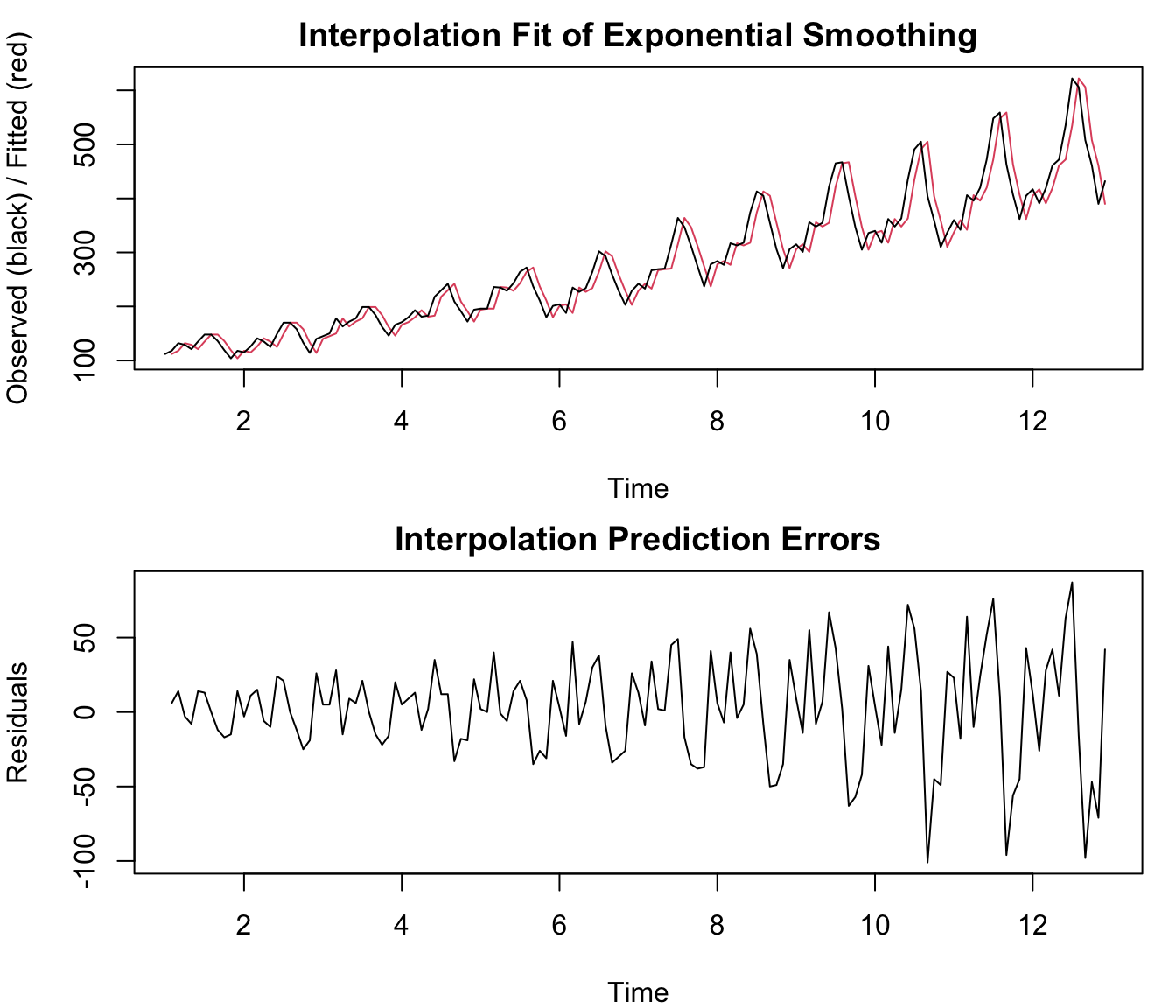
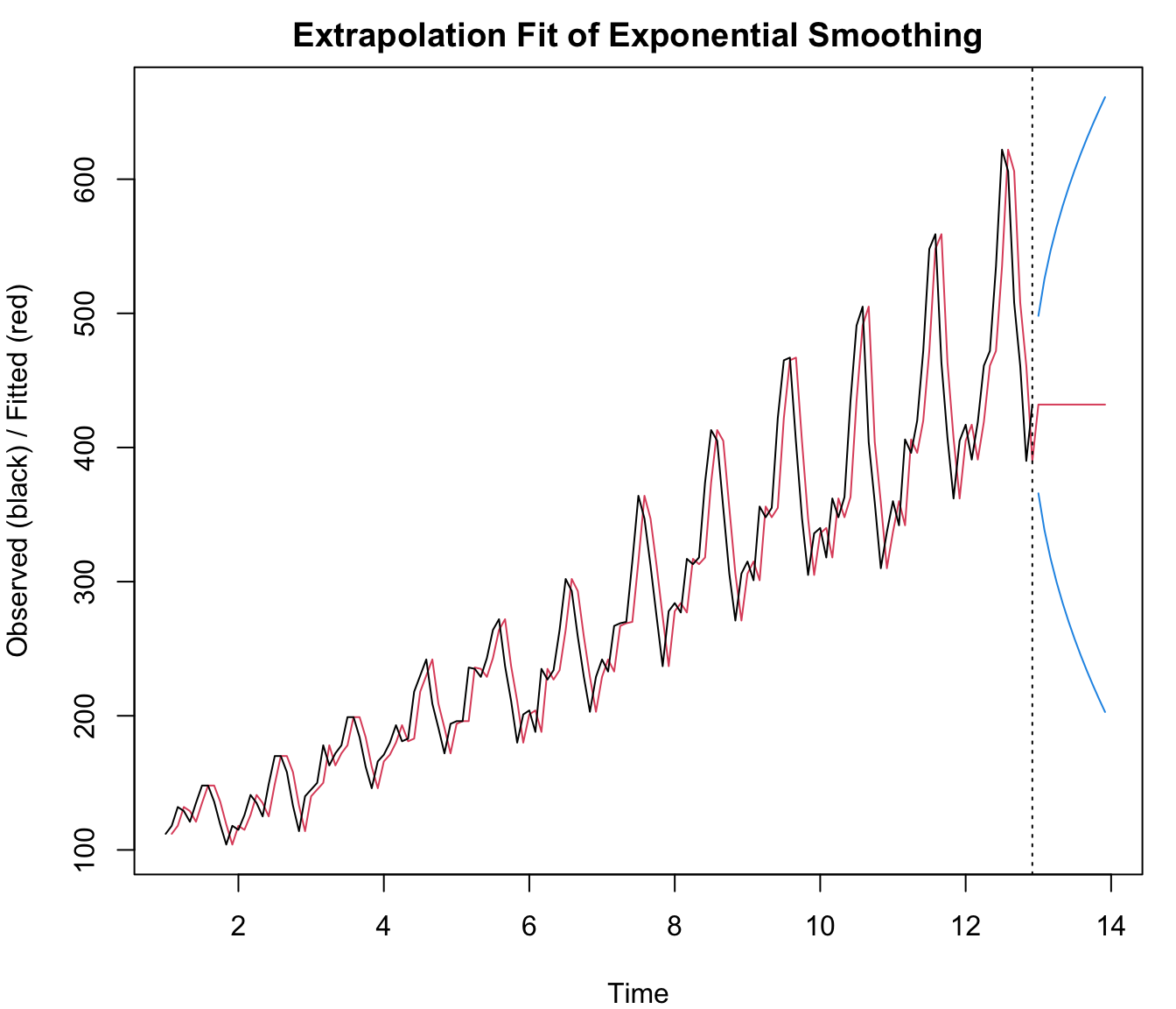
The single exponential smoothing model was fitted to the HPC time series. The Exponential Smoothing R module computes an estimate for \(\hat{\alpha}\), interpolation forecasts \(\hat{Y}_{t \leq T}\), residual diagnostics, and extrapolation forecasts \(\hat{Y}_{t>T}\):

• https://shiny.wessa.net/expsmoothing/
• RFC: menu item Time Series / Exponential Smoothing

The computational results show that the smoothing constant is \(\hat{\alpha} \simeq 0.28\) and the forecast \(\hat{Y}_{T+h} \simeq 20228\) (million USD). The forecast on the long-run is a “flat line” because the model is (seemingly) not able to cope with trends. In addition, the model is - for obvious reasons - unable to predict seasonal fluctuations.

Interactive Shiny app (click to load).

Open in new tab

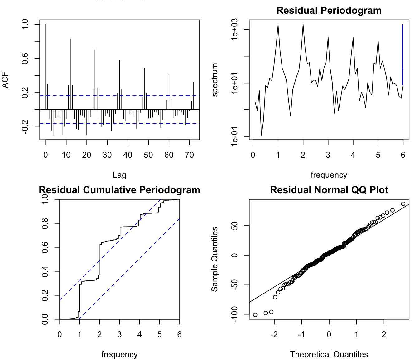
From the residual diagnostics (the residual ACF, spectrum, and cumulative periodogram) that are displayed in the output, it is obvious that a strong, seasonal pattern is present in the prediction errors. This means that the model should be improved by adding a long-run trend and seasonal component to the forecasting model. For background on these diagnostics, see the (P)ACF chapter (PACF.qmd) and Chapter 93.

147.2.4.3 Interpretation

The single exponential smoothing model has been criticized because it seems to be unable to adequately model trend-like behavior. This criticism is not necessarily justified - depending on how “trend-like behavior” is defined. To understand this let us consider the special case where \(\alpha = 1\) which corresponds to the Random Walk model. In finance, the efficient market hypothesis (EMH) (Fama 1970) implies (under strong assumptions) that stock market prices behave approximately like a Random Walk: all relevant information is quickly reflected in the last known stock prices. If the EMH is true then it implies that the best prediction that can be made about future prices is the current price: \(Y_t = Y_{t-1} + e_t \Rightarrow \hat{Y_t} = Y_{t-1}\). If we carefully examine stock price time series then we observe that all of them exhibit long-run trends (which can be easily verified through decomposition or analysis of the ACF or spectrum).

In other words, the EMH is often associated with stock prices behaving approximately as a random walk (possibly with drift), where the one-step-ahead forecast is the latest observed price. This is compatible with the naive forecast and with the \(\alpha = 1\) special case of single exponential smoothing, but it does not imply that SES is the only valid model or that all stock series share the same long-run trend structure. Ultimately, this implies that some types of long-run trends cannot be predicted - in these cases a single exponential smoothing model might not be a bad choice. From the empirical evidence that we have seen about the HPC time series however, it is obvious that the long-run trend is positive - hence, we expect the forecast to behave similarly. If we make an explicit distinction between the “level” of the time series and its incremental “trend” then it is fair to say that single exponential smoothing only models the “level” (and not the “trend”). If we treat both components as one then we need to make a distinction between trends that are predictable (like in retail sales) and trends that are unpredictable (like efficient stock markets).

Another remark about the trend in a single exponential smoothing model is related to the fact that it is possible to model a “deterministic” trend by simply adding a constant term to the equation (which is estimated together with the smoothing constant). The reason why this is the case and how this is interpreted, is beyond the scope of this document.

147.2.4.4 Conclusion

The HPC time series should not be modeled by single exponential smoothing. An “incremental” trend and a seasonal component needs to be added (which requires a more sophisticated model).

If you prefer to compute the Single Exponential Smoothing Model on your local machine, the following script can be used in the R console:

Note: the local script below uses AirPassengers as a generic template dataset. The embedded app and chapter interpretation use the HPC series, so numeric outputs will differ unless you replace x with the HPC data.

par(mar = c(4, 4, 2, 1))
x <- AirPassengers
par1 = 12 #Seasonal period
par2 = 'Single' #Type of Exponential Smoothing
par3 = 'additive' #Type of seasonality
par4 = 12 #Number of Forecasts
if (par2 == 'Single') K <- 1
if (par2 == 'Double') K <- 2
if (par2 == 'Triple') K <- par1
nx <- length(x)
nxmK <- nx - K
x <- ts(x, frequency = par1)
if (par2 == 'Single') fit <- HoltWinters(x, gamma=F, beta=F)
if (par2 == 'Double') fit <- HoltWinters(x, gamma=F)
if (par2 == 'Triple') fit <- HoltWinters(x, seasonal=par3)
print(fit)
print(fit$fitted)
(myresid <- x - fit$fitted[,'xhat'])
op <- par(mfrow=c(2,1))
plot(fit,ylab='Observed (black) / Fitted (red)',main='Interpolation Fit of Exponential Smoothing')
plot(myresid,ylab='Residuals',main='Interpolation Prediction Errors')

par(op)
p <- predict(fit, par4, prediction.interval=TRUE)
np <- length(p[,1])
plot(fit,p,ylab='Observed (black) / Fitted (red)',main='Extrapolation Fit of Exponential Smoothing')

print(p)
op <- par(mfrow = c(2,2))
acf(as.numeric(myresid),lag.max = nx/2,main='Residual ACF')
spectrum(myresid,main='Residual Periodogram')
cpgram(myresid,main='Residual Cumulative Periodogram')
qqnorm(myresid,main='Residual Normal QQ Plot')
qqline(myresid)

par(op)

Holt-Winters exponential smoothing without trend and without seasonal component.

Call:
HoltWinters(x = x, beta = F, gamma = F)

Smoothing parameters:
 alpha: 0.9999339
 beta : FALSE
 gamma: FALSE

Coefficients:
      [,1]
a 431.9972
           xhat    level
Feb  1 112.0000 112.0000
Mar  1 117.9996 117.9996
Apr  1 131.9991 131.9991
May  1 129.0002 129.0002
Jun  1 121.0005 121.0005
Jul  1 134.9991 134.9991
Aug  1 147.9991 147.9991
Sep  1 148.0000 148.0000
Oct  1 136.0008 136.0008
Nov  1 119.0011 119.0011
Dec  1 104.0010 104.0010
Jan  2 117.9991 117.9991
Feb  2 115.0002 115.0002
Mar  2 125.9993 125.9993
Apr  2 140.9990 140.9990
May  2 135.0004 135.0004
Jun  2 125.0007 125.0007
Jul  2 148.9984 148.9984
Aug  2 169.9986 169.9986
Sep  2 170.0000 170.0000
Oct  2 158.0008 158.0008
Nov  2 133.0017 133.0017
Dec  2 114.0013 114.0013
Jan  3 139.9983 139.9983
Feb  3 144.9997 144.9997
Mar  3 149.9997 149.9997
Apr  3 177.9981 177.9981
May  3 163.0010 163.0010
Jun  3 171.9994 171.9994
Jul  3 177.9996 177.9996
Aug  3 198.9986 198.9986
Sep  3 199.0000 199.0000
Oct  3 184.0010 184.0010
Nov  3 162.0015 162.0015
Dec  3 146.0011 146.0011
Jan  4 165.9987 165.9987
Feb  4 170.9997 170.9997
Mar  4 179.9994 179.9994
Apr  4 192.9991 192.9991
May  4 181.0008 181.0008
Jun  4 182.9999 182.9999
Jul  4 217.9977 217.9977
Aug  4 229.9992 229.9992
Sep  4 241.9992 241.9992
Oct  4 209.0022 209.0022
Nov  4 191.0012 191.0012
Dec  4 172.0013 172.0013
Jan  5 193.9985 193.9985
Feb  5 195.9999 195.9999
Mar  5 196.0000 196.0000
Apr  5 235.9974 235.9974
May  5 235.0001 235.0001
Jun  5 229.0004 229.0004
Jul  5 242.9991 242.9991
Aug  5 263.9986 263.9986
Sep  5 271.9995 271.9995
Oct  5 237.0023 237.0023
Nov  5 211.0017 211.0017
Dec  5 180.0020 180.0020
Jan  6 200.9986 200.9986
Feb  6 203.9998 203.9998
Mar  6 188.0011 188.0011
Apr  6 234.9969 234.9969
May  6 227.0005 227.0005
Jun  6 233.9995 233.9995
Jul  6 263.9980 263.9980
Aug  6 301.9975 301.9975
Sep  6 293.0006 293.0006
Oct  6 259.0022 259.0022
Nov  6 229.0020 229.0020
Dec  6 203.0017 203.0017
Jan  7 228.9983 228.9983
Feb  7 241.9991 241.9991
Mar  7 233.0006 233.0006
Apr  7 266.9978 266.9978
May  7 268.9999 268.9999
Jun  7 269.9999 269.9999
Jul  7 314.9970 314.9970
Aug  7 363.9968 363.9968
Sep  7 347.0011 347.0011
Oct  7 312.0023 312.0023
Nov  7 274.0025 274.0025
Dec  7 237.0024 237.0024
Jan  8 277.9973 277.9973
Feb  8 283.9996 283.9996
Mar  8 277.0005 277.0005
Apr  8 316.9974 316.9974
May  8 313.0003 313.0003
Jun  8 317.9997 317.9997
Jul  8 373.9963 373.9963
Aug  8 412.9974 412.9974
Sep  8 405.0005 405.0005
Oct  8 355.0033 355.0033
Nov  8 306.0032 306.0032
Dec  8 271.0023 271.0023
Jan  9 305.9977 305.9977
Feb  9 314.9994 314.9994
Mar  9 301.0009 301.0009
Apr  9 355.9964 355.9964
May  9 348.0005 348.0005
Jun  9 354.9995 354.9995
Jul  9 421.9956 421.9956
Aug  9 464.9972 464.9972
Sep  9 466.9999 466.9999
Oct  9 404.0042 404.0042
Nov  9 347.0038 347.0038
Dec  9 305.0028 305.0028
Jan 10 335.9980 335.9980
Feb 10 339.9997 339.9997
Mar 10 318.0015 318.0015
Apr 10 361.9971 361.9971
May 10 348.0009 348.0009
Jun 10 362.9990 362.9990
Jul 10 434.9952 434.9952
Aug 10 490.9963 490.9963
Sep 10 504.9991 504.9991
Oct 10 404.0067 404.0067
Nov 10 359.0030 359.0030
Dec 10 310.0032 310.0032
Jan 11 336.9982 336.9982
Feb 11 359.9985 359.9985
Mar 11 342.0012 342.0012
Apr 11 405.9958 405.9958
May 11 396.0007 396.0007
Jun 11 419.9984 419.9984
Jul 11 471.9966 471.9966
Aug 11 547.9950 547.9950
Sep 11 558.9993 558.9993
Oct 11 463.0063 463.0063
Nov 11 407.0037 407.0037
Dec 11 362.0030 362.0030
Jan 12 404.9972 404.9972
Feb 12 416.9992 416.9992
Mar 12 391.0017 391.0017
Apr 12 418.9981 418.9981
May 12 460.9972 460.9972
Jun 12 471.9993 471.9993
Jul 12 534.9958 534.9958
Aug 12 621.9942 621.9942
Sep 12 606.0011 606.0011
Oct 12 508.0065 508.0065
Nov 12 461.0031 461.0031
Dec 12 390.0047 390.0047
             Jan           Feb           Mar           Apr           May
1                 6.000000e+00  1.400040e+01 -2.999074e+00 -8.000198e+00
2  -2.999075e+00  1.099980e+01  1.500073e+01 -5.999008e+00 -1.000040e+01
3   5.001719e+00  5.000331e+00  2.800033e+01 -1.499815e+01  8.999009e+00
4   5.001322e+00  9.000331e+00  1.300059e+01 -1.199914e+01  1.999207e+00
5   2.001454e+00  1.323101e-04  4.000000e+01 -9.973557e-01 -6.000066e+00
6   3.001388e+00 -1.599980e+01  4.699894e+01 -7.996893e+00  6.999471e+00
7   1.300172e+01 -8.999140e+00  3.399941e+01  2.002248e+00  1.000132e+00
8   6.002710e+00 -6.999603e+00  3.999954e+01 -3.997356e+00  4.999736e+00
9   9.002314e+00 -1.399940e+01  5.499907e+01 -7.996364e+00  6.999471e+00
10  4.002049e+00 -2.199974e+01  4.399855e+01 -1.399709e+01  1.499907e+01
11  2.300178e+01 -1.799848e+01  6.399881e+01 -9.995769e+00  2.399934e+01
12  1.200284e+01 -2.599921e+01  2.799828e+01  4.200185e+01  1.100278e+01
             Jun           Jul           Aug           Sep           Oct
1   1.399947e+01  1.300093e+01  8.594517e-04 -1.200000e+01 -1.700079e+01
2   2.399934e+01  2.100159e+01  1.388351e-03 -1.200000e+01 -2.500079e+01
3   6.000595e+00  2.100040e+01  1.388272e-03 -1.500000e+01 -2.200099e+01
4   3.500013e+01  1.200231e+01  1.200079e+01 -3.299921e+01 -1.800218e+01
5   1.399960e+01  2.100093e+01  8.001388e+00 -3.499947e+01 -2.600231e+01
6   3.000046e+01  3.800198e+01 -8.997488e+00 -3.400059e+01 -3.000225e+01
7   4.500007e+01  4.900297e+01 -1.699676e+01 -3.500112e+01 -3.800231e+01
8   5.600033e+01  3.900370e+01 -7.997422e+00 -5.000053e+01 -4.900331e+01
9   6.700046e+01  4.300443e+01  2.002843e+00 -6.299987e+01 -5.700416e+01
10  7.200099e+01  5.600476e+01  1.400370e+01 -1.009991e+02 -4.500668e+01
11  5.200159e+01  7.600344e+01  1.100502e+01 -9.599927e+01 -5.600635e+01
12  6.300073e+01  8.700416e+01 -1.599425e+01 -9.800106e+01 -4.700648e+01
             Nov           Dec
1  -1.500112e+01  1.399901e+01
2  -1.900165e+01  2.599874e+01
3  -1.600145e+01  1.999894e+01
4  -1.900119e+01  2.199874e+01
5  -3.100172e+01  2.099795e+01
6  -2.600198e+01  2.599828e+01
7  -3.700251e+01  4.099755e+01
8  -3.500324e+01  3.499769e+01
9  -4.200377e+01  3.099722e+01
10 -4.900298e+01  2.699676e+01
11 -4.500370e+01  4.299702e+01
12 -7.100311e+01  4.199531e+01
            fit      upr      lwr
Jan 13 431.9972 498.1557 365.8387
Feb 13 431.9972 525.5564 338.4381
Mar 13 431.9972 546.5821 317.4124
Apr 13 431.9972 564.3077 299.6868
May 13 431.9972 579.9243 284.0701
Jun 13 431.9972 594.0429 269.9516
Jul 13 431.9972 607.0262 256.9682
Aug 13 431.9972 619.1109 244.8836
Sep 13 431.9972 630.4611 233.5334
Oct 13 431.9972 641.1963 222.7981
Nov 13 431.9972 651.4070 212.5875
Dec 13 431.9972 661.1631 202.8313

To compute the Double or Triple Exponential Smoothing Model, one simply has to change the second parameter (par2). In the case of Triple Exponential Smoothing it also possible to specify “multiplicative” instead of “additive”.

147.2.5 Double Exponential Smoothing

147.2.5.1 Model

This model applies single exponential smoothing twice (with two different smoothing constants⁶ \(\alpha\) and \(\beta\)), following Holt’s extension for trend Holt (1957), which leads to \(\hat{Y}_{t+h} = A_t + h B_t\) where

\[ \left\{ \begin{array}{l}A_t = \alpha Y_t + (1-\alpha) (A_{t-1} + B_{t-1})\\B_t = \beta (A_t - A_{t-1}) + (1-\beta) B_{t-1} \\\end{array} \right. \]

with \(0 < \alpha \leq 1\) and \(0 < \beta \leq 1\).

147.2.5.2 Analysis

The double exponential smoothing model was fitted to the HPC time series. The Exponential Smoothing R module computes an estimate for \(\hat{\alpha}\), \(\hat{\beta}\), interpolation forecasts \(\hat{Y}_{t \leq T}\), residual diagnostics, and extrapolation forecasts \(\hat{Y}_{t>T}\).

Interactive Shiny app (click to load).

Open in new tab

The results lead to much better (i.e. more realistic) predictions than the previous model.

The problem with this model is that it still does not fit our HPC time series well. This is due to the fact that it doesn’t include a seasonal component which can be clearly seen in the residual ACF, spectrum and cumulative periodogram.

147.2.6 Triple Exponential Smoothing (Holt-Winters model)

147.2.6.1 Model

The Holt-Winters model includes a level, an (incremental) trend, and a seasonal component. For each component there is a parameter (\(\alpha\), \(\beta\), and \(\gamma\)) that characterizes the underlying dynamics of the time series. The model comes in two flavors, depending on the relationship between the level and seasonality⁷, and follows Winters’ seasonal extension of exponential smoothing Winters (1960).

The additive Holt-Winters model is defined by the following relationships:

\[ \hat{Y}_{t+h} = A_t + h B_t + S_{t+h-s} \]

where

\[ \begin{align*}\left\{ \begin{array}{l}A_t = \alpha (Y_t - S_{t-s}) + (1-\alpha) (A_{t-1} + B_{t-1})\\B_t = \beta (A_t - A_{t-1}) + (1-\beta) B_{t-1} \\S_t = \gamma (Y_t - A_t) + (1-\gamma) S_{t-s}\\\end{array} \right.\end{align*} \]

The multiplicative Holt-Winters model is defined by the following relationships:

\[ \hat{Y}_{t+h} = \left( A_t + h B_t \right) S_{t+h-s} \]

where

\[ \begin{align*}\left\{ \begin{array}{l}A_t = \alpha (Y_t / S_{t-s}) + (1-\alpha) (A_{t-1} + B_{t-1})\\B_t = \beta (A_t - A_{t-1}) + (1-\beta) B_{t-1} \\S_t = \gamma (Y_t / A_t) + (1-\gamma) S_{t-s}\\\end{array} \right.\end{align*} \]

Single exponential smoothing (\(\beta = \gamma = 0\)) and double exponential smoothing (\(\gamma = 0\)) are both special cases of the additive Holt-Winters model.

147.2.6.2 Analysis

The triple exponential smoothing model was fitted to the HPC time series by the use of the Exponential Smoothing R module. The results show improved extrapolation forecasts and residual diagnostics.

Interactive Shiny app (click to load).

Open in new tab

In the ACF, spectrum and cumulative periodogram there is no clear evidence of residual seasonality, which suggests that the model captures seasonal effects adequately. In addition, the Normal QQ plot suggests that residuals are approximately normally distributed. The model is not perfect because the residual ACF still exhibits a non-random (regular) autocorrelation pattern \(\hat{\rho}_{k \in \left\{ 3, 6, 9, … \right\}} > 0\) and \(\hat{\rho}_{k \in \left\{ 1, 4, 7, … \right\}} < 0\).

147.2.6.3 Assignment

Examine the multiplicative Holt-Winters model and compare the results with the additive model. Which model is better?

Box, George E. P., and Gwilym M. Jenkins. 1970. Time Series Analysis: Forecasting and Control. San Francisco: Holden-Day.

Brown, Robert G. 1959. Statistical Forecasting for Inventory Control. New York: McGraw-Hill.

Fama, Eugene F. 1970. “Efficient Capital Markets: A Review of Empirical Work.” The Journal of Finance 25 (2): 383–417.

Holt, Charles C. 1957. “Forecasting Seasonals and Trends by Exponentially Weighted Moving Averages.” Research Memorandum 52. Pittsburgh, PA: Office of Naval Research.

Winters, Peter R. 1960. “Forecasting Sales by Exponentially Weighted Moving Averages.” Management Science 6 (3): 324–42. https://doi.org/10.1287/mnsc.6.3.324.

---

1. In this case \(s=12\) because we use monthly data

2. Note that in the R module the seasonal dummies are denoted by M or S instead of D.

3. We actually know that the 12th observation corresponds to the month of December because the HPC time series starts in January 2001.

4. Actually, we can use any measure of central tendency - not just the arithmetic mean.

5. Sometimes this model is also called ARIMA(0,1,1) which is consistent with the work of Box & Jenkins (Box and Jenkins 1970) where the more general class of ARIMA forecasting models is discussed.

6. Note that in some textbooks this model is defined with only one parameter - in other words: \(\alpha = \beta\). We don’t want to impose this restriction on the parameters.

7. Again, the difference between the additive and multiplicative models is related to the Heteroskedasticity problem.