When \(n\) bivariate normal observations are drawn under zero population correlation (\(\rho = 0\)), the sample correlation coefficient \(r\) follows a specific symmetric distribution on \((-1, 1)\). This sampling distribution provides the exact basis for testing whether an observed correlation is statistically distinguishable from zero.
Formally, when \((X_i, Y_i)\) are i.i.d. bivariate Normal with correlation \(\rho = 0\), the sample Pearson correlation \(R\) defined on \((-1, 1)\) follows the distribution \(R \sim \text{CorDist}(n)\) with sample size \(n \geq 3\).
Note: This chapter describes the distribution of the sample correlation under \(H_0: \rho = 0\). For the full hypothesis test of \(H_0: \rho = 0\), including software output and interpretation, see Chapter 71.
WarningScope and Applicability
This distribution applies to Pearson correlation computed from i.i.d. paired observations under a bivariate Normal model and the null hypothesis \(H_0:\rho = 0\). It should not be used for sample autocorrelations of a single time series, nor for correlations between serially dependent time series. In those settings, inference is usually based on large-sample approximations such as white-noise confidence bands, Bartlett-type formulas, or large-lag variance results rather than the exact finite-sample distribution described here.
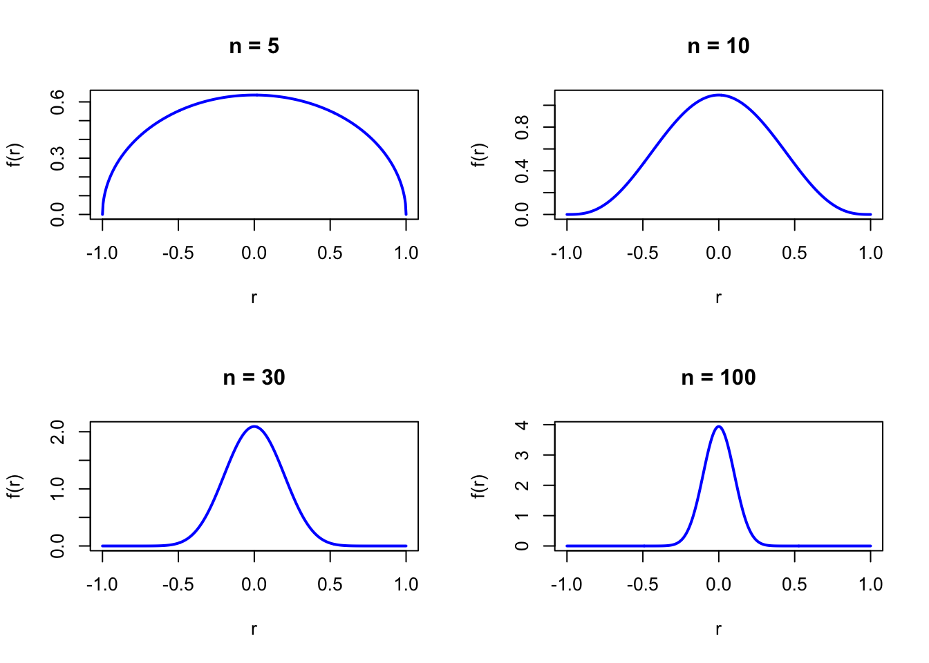
The figure below shows examples of the sample correlation distribution for different sample sizes.
Code
dcorr <-function(r, n) {ifelse(abs(r) <1, (1- r^2)^((n -4)/2) /beta(0.5, (n -2)/2),0)}par(mfrow =c(2, 2))r <-seq(-1, 1, length =500)plot(r, dcorr(r, 5), type ="l", lwd =2, col ="blue",xlab ="r", ylab ="f(r)", main ="n = 5")plot(r, dcorr(r, 10), type ="l", lwd =2, col ="blue",xlab ="r", ylab ="f(r)", main ="n = 10")plot(r, dcorr(r, 30), type ="l", lwd =2, col ="blue",xlab ="r", ylab ="f(r)", main ="n = 30")plot(r, dcorr(r, 100), type ="l", lwd =2, col ="blue",xlab ="r", ylab ="f(r)", main ="n = 100")par(mfrow =c(1, 1))
Figure 43.1: Sampling distribution of Pearson r under H0: rho = 0 for various sample sizes
43.2 Purpose
The sample correlation distribution serves as the null reference distribution for testing independence between two continuous variables in a bivariate normal population. It enables exact inference for any sample size \(n \geq 3\) without requiring large-sample approximations. Common applications include:
Testing whether two continuous variables are linearly uncorrelated in a bivariate normal population
Determining critical values for the Pearson correlation test statistic
Computing exact p-values for observed correlations under \(H_0: \rho = 0\)
Understanding the sampling variability of \(r\) when the true correlation is zero
Teaching the foundations of correlation hypothesis testing
Relation to the discrete setting. This is an inferential tool, not a data-generating model. Its closest discrete analog is the distribution of a sample proportion under \(H_0: p = 0.5\), which is also symmetric and used for hypothesis testing of association.
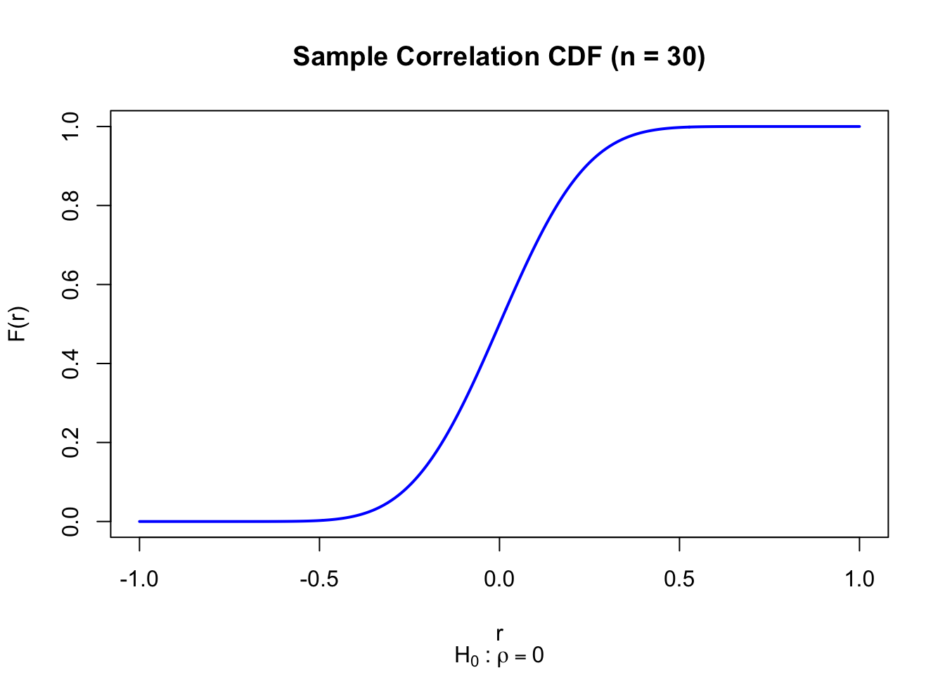
43.3 Distribution Function
The CDF is obtained via the regularized incomplete beta function. In R:
For large \(n\), \(g_2 \to 3\) (approaching the Normal), consistent with the asymptotic normality of \(r\).
43.18 Key Result: t-Transform
The test statistic
\[
T = \frac{R\sqrt{n-2}}{\sqrt{1-R^2}}
\]
follows a \(t\)-distribution with \(n-2\) degrees of freedom under \(H_0: \rho = 0\) (see Chapter 25). This is the most commonly used result for testing correlation.
43.19 Parameter Estimation
The sample correlation coefficient \(r = \sum(x_i-\bar x)(y_i - \bar y) / \sqrt{\sum(x_i-\bar x)^2\sum(y_i-\bar y)^2}\) is computed directly from data. The parameter \(n\) is the sample size.
43.20 R Module
43.20.1 RFC
The sample correlation distribution is covered in the context of the correlation test: see the “Hypothesis Testing / Pearson Correlation Test” module in RFC.
Sample correlations under \(H_0: \rho = 0\) can be simulated by generating bivariate normal data with zero correlation and computing the sample correlation:
set.seed(123)n <-30; N_sim <-1000# Simulate N_sim sample correlations under H0: rho = 0r_sims <-replicate(N_sim, { x <-rnorm(n); y <-rnorm(n)cor(x, y)})cat("Simulated mean of r:", round(mean(r_sims), 4), "\n")cat("Theoretical mean:", 0, "\n")cat("Simulated var of r:", round(var(r_sims), 4), "\n")cat("Theoretical var:", round(1/(n-1), 4), "\n")
Simulated mean of r: 0.006
Theoretical mean: 0
Simulated var of r: 0.0357
Theoretical var: 0.0345